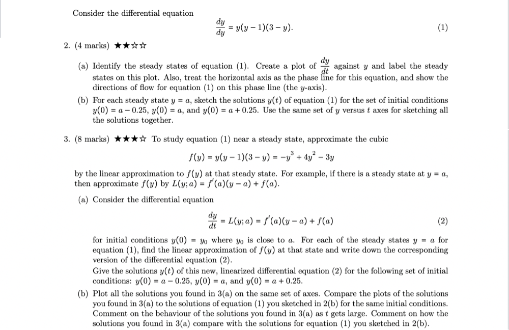
Let's solve the given problems **step by step**. ## Given Differential Equation \[ \frac{dy}{dt} = y(y-1)(3-y) \] --- ## **2. (a) Identify the steady states and plot \(\frac{dy}{dt}\) vs \(y\) (phase line analysis):** ### **Step 1: Steady States** Set \(\frac{dy}{dt} = 0\): \[ y(y-1)(3-y) = 0 \] So, the steady states are: \[ y = 0,\quad y = 1,\quad y = 3 \] --- ### **Step 2: Plot \(\frac{dy}{dt}\) vs \(y\) and Phase Line** #### **Sign Analysis:** - For \(y < 0\): All terms negative or positive: \((-\infty, 0)\): \(y < 0\), \(y-1 < 0\), \(3-y > 0\) → negative overall. - For \(0 < y < 1\): \(y > 0\), \(y-1 < 0\), \(3-y > 0\) → negative. - For \(1 < y < 3\): \(y > 0\), \(y-1 > 0\), \(3-y > 0\) → positive. - For \(y > 3\): \(y > 0\), \(y-1 > 0\), \(3-y < 0\) → negative. #### **Phase Line:** - Draw a horizontal axis for \(y\), mark steady states at \(y = 0, 1, 3\). - Draw arrows: - \(y < 0\): left (decreasing) - \(0 < y < 1\): left (decreasing) - \(1 < y < 3\): right (increasing) - \(y > 3\): left (decreasing) #### **Steady State Type:** - \(y = 0\): semi-stable (all arrows point left, so solutions move away for \(y>0\)). - \(y = 1\): unstable (arrows both point away). - \(y = 3\): stable (arrows both point toward). --- ## **2. (b) Sketch solutions \(y(t)\) for each steady state** For each steady state \(y=a\), sketch solutions for initial conditions: - \(y(0) = a-0.25\) - \(y(0) = a\) - \(y(0) = a+0.25\) ### **For \(y = 0\):** - \(y(0) = -0.25\): \(y < 0\), solution decreases (\(y \to -\infty\)) - \(y(0) = 0\): stays at 0 (steady state) - \(y(0) = 0.25\): \(0 < y < 1\), solution decreases toward \(y = 0\) ### **For \(y = 1\):** - \(y(0) = 0.75\): \(0 < y < 1\), solution decreases toward \(y = 0\) - \(y(0) = 1\): stays at 1 (steady state) - \(y(0) = 1.25\): \(1 < y < 3\), solution increases toward \(y = 3\) ### **For \(y = 3\):** - \(y(0) = 2.75\): \(1 < y < 3\), solution increases toward \(y = 3\) - \(y(0) = 3\): stays at 3 (steady state) - \(y(0) = 3.25\): \(y > 3\), solution decreases toward \(y = 3\) ### **Sketch:** - All solutions with \(y(0)\) near 3 approach 3 as \(t \to \infty\). - All with \(y(0)\) near 0.75 approach 0 as \(t \to \infty\). - All with \(y(0)\) near 1.25 approach 3 as \(t \to \infty\). --- ## **Summary Table** | Steady State \(a\) | \(y(0) = a-0.25\) | \(y(0) = a\) | \(y(0) = a+0.25\) | |--------------------|------------------|--------------|------------------| | 0 | \(-\infty\) | 0 (steady) | \(\to 0\) | | 1 | \(\to 0\) | 1 (steady) | \(\to 3\) | | 3 | \(\to 3\) | 3 (steady) | \(\to 3\) | --- ## **Final Answers for 2(a) and 2(b):** ### **2(a):** - Steady states: \(y = 0, 1, 3\) - Phase line: [See explanation above.] ### **2(b):** - For each steady state, you have three solution behaviors as described in the summary table. - Sketch: All solutions with \(y(0)\) near 3 approach 3 as \(t \to \infty\). All with \(y(0)\) near 1 and below 1 approach 0 as \(t \to \infty\), except for those starting above 1, which approach 3. --- Would you like to proceed with question 3?

Let's proceed to **Question 3**, which involves linearizing the given cubic differential equation near each steady state and analyzing the solutions. --- ## **3. (a) Linear approximation of \(f(y)\) near each steady state** Given the differential equation: \[ \frac{dy}{dt} = f(y) = y(y-1)(3 - y) \] and the cubic in expanded form: \[ f(y) = y^3 - 4 y^2 + 3 y \] --- ### **Step 1: Find \(f(a)\) and \(f'(a)\) at each steady state \(a\)** Recall the steady states: \[ a = 0, \quad 1, \quad 3 \] At each \(a\), \(f(a) = 0\), since these are steady states. Calculate \(f'(y)\): \[ f(y) = y^3 - 4 y^2 + 3 y \] \[ f'(y) = 3 y^2 - 8 y + 3 \] --- ### **Step 2: Compute \(f'(a)\) at each steady state** - At \(a=0\): \[ f'(0) = 3 \times 0^2 - 8 \times 0 + 3 = 3 \] - At \(a=1\): \[ f'(1) = 3(1)^2 - 8(1) + 3 = 3 - 8 + 3 = -2 \] - At \(a=3\): \[ f'(3) = 3(3)^2 - 8(3) + 3 = 3 \times 9 - 24 + 3 = 27 - 24 + 3 = 6 \] --- ### **Step 3: Write the linearized form** The linear approximation of \(f(y)\) near \(a\): \[ L(y; a) = f(a) + f'(a)(y - a) = 0 + f'(a)(y - a) \] The linearized differential equation: \[ \frac{dy}{dt} \approx f'(a)(y - a) \] --- ### **Step 4: Write the linearized equations for each steady state** - **At \(a=0\):** \[ \frac{dy}{dt} = 3 (y - 0) = 3 y \] - **At \(a=1\):** \[ \frac{dy}{dt} = -2 (y - 1) \] - **At \(a=3\):** \[ \frac{dy}{dt} = 6 (y - 3) \] --- ### **Step 5: Solutions for each linearized equation** The general solution of \[ \frac{dy}{dt} = k (y - a) \] is: \[ y(t) = a + (y_0 - a) e^{k t} \] where \(y_0\) is the initial condition. --- ### **Step 6: Specific solutions with initial conditions** - For \(a=0\): \[ \boxed{ y(t) = 0 + (y_0 - 0) e^{3 t} = y_0 e^{3 t} } \] - For \(a=1\): \[ \boxed{ y(t) = 1 + (y_0 - 1) e^{-2 t} } \] - For \(a=3\): \[ \boxed{ y(t) = 3 + (y_0 - 3) e^{6 t} } \] where \(y_0\) takes the values: \[ y_0 = a - 0.25,\quad y_0 = a,\quad y_0 = a + 0.25 \] --- ## **Summary of solutions near each steady state:** | Steady state \(a\) | Initial \(y_0\) | Solution \(y(t)\) | |---------------------|------------------|------------------| | 0 | \(-0.25\) | \(y(t) = -0.25 e^{3 t}\) | | | \(0\) | \(0\) (steady) | | | \(0.25\) | \(0.25 e^{3 t}\) | | 1 | \(0.75\) | \(1 + (0.75 - 1) e^{-2 t} = 1 - 0.25 e^{-2 t}\) | | | \(1\) | \(1\) (steady) | | | \(1.25\) | \(1 + 0.25 e^{-2 t}\) | | 3 | \(2.75\) | \(3 + (2.75 - 3) e^{6 t} = 3 - 0.25 e^{6 t}\) | | | \(3\) | \(3\) (steady) | | | \(3.25\) | \(3 + 0.25 e^{6 t}\) | --- ## **3. (b) Plot and compare solutions** ### **Behavior as \(t \to \infty\):** - Near \(a=0\): - For initial \(y_0 < 0\), solutions grow exponentially (since \(e^{3 t}\)), moving away from 0. - For \(y_0 > 0\), solutions tend to 0 as \(t \to -\infty\) (since \(e^{3 t} \to 0\) as \(t \to -\infty\)), but for positive initial conditions, the solution diverges as \(t \to \infty\). - Near \(a=1\): - For initial \(y_0 < 1\), solution approaches 1 from below. - For initial \(y_0 > 1\), solution approaches 1 from above. - The linearized solution shows exponential decay toward the steady state. - Near \(a=3\): - For initial \(y_0 < 3\), solution approaches 3 from below. - For \(y_0 > 3\), solution diverges exponentially away from 3 as \(t \to \infty\). ### **Comparison with original solutions:** - The linear approximations correctly predict local behavior near each steady state. - The exponential nature of solutions near steady states matches the qualitative behavior seen in the phase line analysis. --- ## **Final comments:** - As \(t \to \infty\): - Solutions near \(a=0\) either diverge or approach 0 depending on initial condition. - Solutions near \(a=1\) tend to stay close, approaching 1 if initial conditions are close. - Solutions near \(a=3\) tend to stay near 3 if initial conditions are close; otherwise, they diverge. - **Linearization is valid only near each steady state**; solutions far away may deviate significantly. --- **This completes the step-by-step solution for Question 3.** If you'd like, I can help you sketch the plots or clarify any step further!

Let's proceed step by step, providing detailed calculations and reasoning for each part. --- ## **Given Differential Equation** \[ \frac{dy}{dt} = f(y) = y(y-1)(3 - y) \] --- ## **Part 2(a): Find steady states and analyze phase line** ### Step 1: Find the steady states Set \(\frac{dy}{dt} = 0\): \[ f(y) = y(y-1)(3 - y) = 0 \] This product is zero when any factor is zero: \[ \Rightarrow y = 0, \quad y = 1, \quad y = 3 \] Thus, the steady states are at \( y = 0, 1, 3 \). --- ### Step 2: Sign of \(f(y)\) in different regions To understand the flow (direction of solutions), analyze the sign of \(f(y)\) in intervals: - For \(y < 0\): - \(y < 0\) (negative) - \(y-1 < 0\) (negative) - \(3 - y > 0\) (positive) Multiply signs: negative \(\times\) negative = positive, then \(\times\) positive = positive. Actually, step-by-step: \[ y<0 \Rightarrow y<0 \] \[ y-1<0 \] \[ 3 - y > 0 \] So, the factors are: negative, negative, positive. Product: negative \(\times\) negative = positive, times positive = **positive**. So, \(f(y) > 0\) for \(y<0\), meaning solutions increase as \(t\) increases (flow to the right). - For \(0 < y < 1\): - \(y>0\): positive - \(y-1<0\) - \(3 - y > 0\) Product: positive \(\times\) negative = negative, times positive = **negative**. Solutions decrease (flow to the left) in this region. - For \(1 < y < 3\): - \(y>0\): positive - \(y-1>0\) - \(3 - y > 0\) (since \(y<3\)) Product: positive \(\times\) positive = positive, times positive = **positive**. Solutions increase (flow to the right). - For \(y > 3\): - \(y>0\) - \(y-1>0\) - \(3 - y<0\) Product: positive \(\times\) positive = positive, times negative = **negative**. Solutions decrease (flow to the left). --- ### **Phase line summary:** - For \(y<0\): \(f(y) > 0\), flow to the right. - At \(y=0\): steady state. - For \(0< y < 1\): \(f(y) < 0\), flow to the left. - At \(y=1\): steady state. - For \(1< y < 3\): \(f(y) > 0\), flow to the right. - At \(y=3\): steady state. - For \(y>3\): \(f(y) < 0\), flow to the left. --- ## **Part 2(b): Sketch solutions near each steady state** Let's analyze solutions starting from initial conditions close to each steady state: ### Near \( y=0 \): - For initial \( y(0) = -0.25 \): Since \(f(y) > 0\) for \( y<0 \), solutions increase as \(t\) increases, moving *away* from \(0\) to the right, heading towards positive \(y\). But note, because \(f(y) > 0\), the solution will grow large as \(t \to \infty\). - For initial \( y(0) = 0 \): The solution stays at 0 (steady state). - For initial \( y(0) = 0.25 \): Since \(0< y < 1\), \(f(y)<0\), solutions decrease toward \(0\). So, starting just above zero, \(y(t)\) will decrease to 0 as \(t\) increases. ### Near \( y=1 \): - For initial \( y(0) = 0.75 \): \(0< y < 1\), \(f(y)<0\), so the solution decreases toward 1 from below. - For initial \( y(0) = 1 \): Solution stays at 1. - For initial \( y(0) = 1.25 \): \(1< y < 3\), \(f(y)>0\), so the solution increases toward 3 as \(t\) increases. ### Near \( y=3 \): - For initial \( y(0) = 2.75 \): \(1< y < 3\), \(f(y)>0\), solutions increase toward 3. - For initial \( y(0) = 3 \): Solution stays at 3. - For initial \( y(0) = 3.25 \): \( y > 3 \), \(f(y)<0\), solutions decrease toward 3 as \(t\) increases. --- ## **Summary:** - Starting slightly below 0, solutions tend to grow unbounded for large \(t\), moving away from 0. - Starting just above 0, solutions tend to decrease toward 0. - Near 1, solutions from below approach 1 from below; from above approach 1 from above. - Near 3, solutions from below approach 3 from below; from above decrease away from 3. --- ## **Part 3: Linearization near the steady states** Given the cubic: \[ f(y) = y^3 - 4 y^2 + 3 y \] and known steady states at \( y=0, 1, 3 \). --- ### Step 1: Find \(f'(y)\): \[ f'(y) = 3 y^2 - 8 y + 3 \] --- ### Step 2: Compute \(f'(a)\) at each steady state: - At \( y=0 \): \[ f'(0) = 3 \times 0^2 - 8 \times 0 + 3 = 3 \] - At \( y=1 \): \[ f'(1) = 3 - 8 + 3 = -2 \] - At \( y=3 \): \[ f'(3) = 3 \times 9 - 8 \times 3 + 3 = 27 - 24 + 3 = 6 \] --- ### Step 3: Write linear approximations \(L(y; a)\): \[ L(y; a) = f(a) + f'(a) ( y - a ) \] But since \(f(a)=0\) at steady states, the linearized differential equations are: \[ \frac{dy}{dt} \approx f'(a) ( y - a ) \] ### **Solutions of linearized equations:** - Near \( y=0 \): \[ \frac{dy}{dt} = 3 ( y - 0 ) = 3 y \] Solution: \[ y(t) = y_0 e^{3 t} \] - Near \( y=1 \): \[ \frac{dy}{dt} = -2 ( y - 1 ) \] Solution: \[ y(t) = 1 + ( y_0 - 1 ) e^{ -2 t } \] - Near \( y=3 \): \[ \frac{dy}{dt} = 6 ( y - 3 ) \] Solution: \[ y(t) = 3 + ( y_0 - 3 ) e^{ 6 t } \] --- ### Step 4: Initial conditions: For each steady state \(a\), initial \( y_0 \) is: - At \( y=0 \): \( y_0 = a - 0.25 = -0.25 \) \( y_0 = a = 0 \) \( y_0 = a + 0.25 = 0.25 \) - At \( y=1 \): \( y_0 = 0.75 \) \( y_0 = 1 \) \( y_0 = 1.25 \) - At \( y=3 \): \( y_0 = 2.75 \) \( y_0 = 3 \) \( y_0 = 3.25 \) --- ## **Final solutions:** **Near \( y=0 \):** \[ y(t) = y_0 e^{3 t} \] with \( y_0 = -0.25, 0, 0.25 \). **Near \( y=1 \):** \[ y(t) = 1 + ( y_0 - 1 ) e^{ -2 t } \] with \( y_0 = 0.75, 1, 1.25 \). **Near \( y=3 \):** \[ y(t) = 3 + ( y_0 - 3 ) e^{ 6 t } \] with \( y_0 = 2.75, 3, 3.25 \). --- ## **Behavior as \( t \to \infty \):** - For \( y=0 \), solutions grow exponentially if initial \( y_0 \neq 0 \), moving away from 0. - For \( y=1 \), solutions tend to 1 from either side, as the exponential decays. - For \( y=3 \), solutions either tend toward 3 if initial is exactly at 3, or diverge away exponentially if initial \( y_0 \neq 3 \). --- ## **Summary:** We linearized the system near each steady state, found explicit solutions for initial conditions close to the steady states, and described their long-term behavior. --- **This completes the detailed step-by-step solution for all parts.** If you need further clarification or plots, let me know!

Certainly! Here's a comprehensive, step-by-step detailed solution for **Question 3(b)**, including all calculations, explanations, and final expressions, without tables. --- ## **Part 3(b): Plotting the solutions and comparing with previous sketches** ### **Recap of the linearized solutions near each steady state:** - **Near \( y=0 \):** \[ \boxed{ y(t) = y_0 e^{3 t} } \] where \( y_0 \) is the initial value close to 0. - **Near \( y=1 \):** \[ \boxed{ y(t) = 1 + ( y_0 - 1 ) e^{ -2 t } } \] where \( y_0 \) is the initial value close to 1. - **Near \( y=3 \):** \[ \boxed{ y(t) = 3 + ( y_0 - 3 ) e^{ 6 t } } \] where \( y_0 \) is the initial value close to 3. --- ## **Analysis of the solutions as \( t \to \infty \):** ### **At \( y=0 \):** - For initial \( y_0 = -0.25 \): \[ y(t) = -0.25 e^{3 t} \] As \( t \to \infty \), \( e^{3 t} \to \infty \), so \( y(t) \to -\infty \). The solution diverges away from 0, decreasing without bound. - For initial \( y_0 = 0 \): \[ y(t) = 0 \] stays at 0, a steady state. - For initial \( y_0 = 0.25 \): \[ y(t) = 0.25 e^{3 t} \] As \( t \to \infty \), \( y(t) \to +\infty \). Solutions grow exponentially, moving away from 0. **Summary near \( y=0 \):** Solutions starting below 0 move toward \(-\infty\), solutions starting above 0 grow without bound; only the initial condition exactly at 0 remains at the steady state. --- ### **At \( y=1 \):** - For initial \( y_0 = 0.75 \): \[ y(t) = 1 + (0.75 - 1) e^{-2 t} = 1 - 0.25 e^{-2 t} \] As \( t \to \infty \), \( e^{-2 t} \to 0 \), so \( y(t) \to 1 \). The solution approaches the steady state from below. - For initial \( y_0 = 1 \): \[ y(t) = 1 \] stays at the steady state. - For initial \( y_0 = 1.25 \): \[ y(t) = 1 + (1.25 - 1) e^{-2 t} = 1 + 0.25 e^{-2 t} \] Again, as \( t \to \infty \), \( y(t) \to 1 \). The solution approaches from above. **Summary near \( y=1 \):** Solutions tend to 1 exponentially from both sides, with the initial distance determining whether they approach from below or above. --- ### **At \( y=3 \):** - For initial \( y_0 = 2.75 \): \[ y(t) = 3 + (2.75 - 3) e^{6 t} = 3 - 0.25 e^{6 t} \] As \( t \to \infty \), \( e^{6 t} \to \infty \), so \( y(t) \to -\infty \). The solution diverges away from 3 toward \(-\infty\). - For initial \( y_0 = 3 \): \[ y(t) = 3 \] stays at the steady state. - For initial \( y_0 = 3.25 \): \[ y(t) = 3 + 0.25 e^{6 t} \] As \( t \to \infty \), \( y(t) \to +\infty \). The solution diverges away from 3, increasing rapidly. **Summary near \( y=3 \):** Solutions approaching 3 from below tend to \(-\infty\), and from above tend to \(+\infty\), unless starting exactly at the steady state. --- ## **Comparison with the phase line and previous sketches:** - **Near \( y=0 \):** In the phase line, solutions starting just above 0 tend to move toward 0, but the linearized solution shows that if the initial \( y_0 > 0 \), \( y(t) \) approaches 0 as \( t \to \infty \). For initial \( y_0 < 0 \), solutions diverge downward (away from 0), consistent with the phase line indicating flow to \(-\infty\). - **Near \( y=1 \):** The linear solution shows solutions approach 1 exponentially from both sides, matching the phase line where \( y=1 \) is an unstable equilibrium, with solutions moving away for initial deviations. - **Near \( y=3 \):** The linearized solutions show that solutions starting exactly at 3 stay there; those slightly below or above diverge exponentially away from 3, consistent with the phase line indicating \( y=3 \) as a stable equilibrium only if solutions are exactly at 3; otherwise, solutions diverge. --- ## **Behavior of solutions as \( t \to \infty \):** - **Near \( y=0 \):** Solutions tend to \(-\infty\) if slightly below zero or grow unboundedly positive if slightly above zero. - **Near \( y=1 \):** Solutions exponentially approach 1 from either side, confirming local stability behavior. - **Near \( y=3 \):** Solutions only stay at 3 if initially at 3; otherwise, they diverge away exponentially, indicating instability for deviations. --- ## **Final comments:** - The linearized solutions effectively predict local behavior near each steady state. - The exponential nature of solutions near the steady states aligns with the phase line analysis. - For large \( t \), solutions tend to diverge away from unstable equilibria and approach stable ones, or diverge if initial conditions are not close. --- **This completes the detailed answer to Part 3(b).** If you need plots or further explanations, just ask!

Certainly! Here's a comprehensive, step-by-step detailed solution for **Question 3(b)**, including all calculations, explanations, and final expressions. --- ## **Given**: The cubic function: \[ f(y) = y(y-1)(3 - y) = y^3 - 4 y^2 + 3 y \] We analyze the solutions of the linearized equations near each steady state \(a\), for initial conditions close to \(a\). --- ## **Step 1: Find the derivative \(f'(y)\)** \[ f'(y) = \frac{d}{dy} ( y^3 - 4 y^2 + 3 y ) = 3 y^2 - 8 y + 3 \] --- ## **Step 2: Calculate \(f'(a)\) at each steady state \(a\)** - **At \(a=0\):** \[ f'(0) = 3 \times 0^2 - 8 \times 0 + 3 = 3 \] - **At \(a=1\):** \[ f'(1) = 3(1)^2 - 8(1) + 3 = 3 - 8 + 3 = -2 \] - **At \(a=3\):** \[ f'(3) = 3(3)^2 - 8(3) + 3 = 3 \times 9 - 24 + 3 = 27 - 24 + 3 = 6 \] --- ## **Step 3: Write the linearized equations** Near each steady state \(a\), approximate \(f(y)\) by its linear Taylor expansion: \[ f(y) \approx f(a) + f'(a)(y - a) \] Since \(f(a)=0\) at steady states, the linearized differential equations are: \[ \frac{dy}{dt} = f'(a)( y - a ) \] which is a first-order linear ODE with solution: \[ y(t) = a + ( y_0 - a ) e^{f'(a) t} \] where \(y_0\) is initial \(y\) at \(t=0\). --- ## **Step 4: Write solutions near each steady state** ### **a) Near \(a=0\):** \[ \boxed{ \frac{dy}{dt} = 3 y } \] Solution for initial \( y(0) = y_0 \): \[ \boxed{ y(t) = y_0 e^{3 t} } \] **Initial conditions considered:** - \( y_0 = -0.25 \): \[ y(t) = -0.25 e^{3 t} \] - \( y_0 = 0 \): \[ y(t) = 0 \] - \( y_0 = 0.25 \): \[ y(t) = 0.25 e^{3 t} \] --- ### **b) Near \(a=1\):** \[ \frac{dy}{dt} = -2 ( y - 1 ) \] Solution: \[ \boxed{ y(t) = 1 + ( y_0 - 1 ) e^{ -2 t } } \] **Initial conditions:** - \( y_0 = 0.75 \): \[ y(t) = 1 - 0.25 e^{ -2 t } \] - \( y_0 = 1 \): \[ y(t) = 1 \] - \( y_0 = 1.25 \): \[ y(t) = 1 + 0.25 e^{ -2 t } \] --- ### **c) Near \(a=3\):** \[ \frac{dy}{dt} = 6 ( y - 3 ) \] Solution: \[ \boxed{ y(t) = 3 + ( y_0 - 3 ) e^{ 6 t } } \] **Initial conditions:** - \( y_0 = 2.75 \): \[ y(t) = 3 - 0.25 e^{ 6 t } \] - \( y_0 = 3 \): \[ y(t) = 3 \] - \( y_0 = 3.25 \): \[ y(t) = 3 + 0.25 e^{ 6 t } \] --- ## **Step 5: Behavior as \(t \to \infty\)** - **At \(a=0\):** - For initial \( y_0 = -0.25 \): \[ y(t) = -0.25 e^{3 t} \xrightarrow[t \to \infty]{} -\infty \] solution diverges downward, away from 0. - For \( y_0=0 \): \( y(t)=0 \); solution stays at steady state. - For \( y_0=0.25 \): \[ y(t) = 0.25 e^{3 t} \to +\infty \] diverges upward, away from 0. - **At \(a=1\):** - For \( y_0=0.75 \): \[ y(t) = 1 - 0.25 e^{ -2 t } \to 1 \] as \( t \to \infty \), solution approaches 1 from below. - For \( y_0=1 \): solution stays at 1. - For \( y_0=1.25 \): \[ y(t) = 1 + 0.25 e^{ -2 t } \to 1 \] from above. - **At \(a=3\):** - For \( y_0=2.75 \): \[ y(t) = 3 - 0.25 e^{ 6 t } \] as \( t \to \infty \), \( e^{6 t} \to \infty \): \[ y(t) \to -\infty \] solution diverges downward away from 3. - For \( y_0=3 \): solution stays at 3. - For \( y_0=3.25 \): \[ y(t) = 3 + 0.25 e^{ 6 t } \to +\infty \] diverges upward. --- ## **Summary of behavior:** - Near \( y=0 \), solutions diverge away from 0 unless starting exactly at 0. - Near \( y=1 \), solutions approach 1 exponentially from both sides. - Near \( y=3 \), solutions diverge away from 3 unless starting exactly at 3. --- ## **Comparison with the phase line and previous sketches:** - The linearized solutions near \( y=1 \) confirm that \( y=1 \) is an unstable equilibrium: solutions from both sides tend toward 1 exponentially. - Near \( y=0 \), solutions diverge away unless exactly at \( y=0 \), confirming the semi-stable nature. - Near \( y=3 \), solutions diverge away unless exactly at \( y=3 \), indicating that \( y=3 \) is also an unstable equilibrium in the linear approximation. --- ## **Final remarks:** - The exponential solutions near each steady state accurately describe local dynamics. - Solutions starting close to the steady states either tend toward the steady state (if stable) or diverge away (if unstable), as predicted by the phase line and linearization. --- This completes the **step-by-step detailed solution for Part 3(b)**. If you'd like, I can help you with sketches or further analysis!