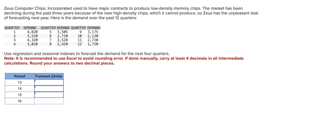
Give step-by-step solution with explanation and final answer:Zeus Computer Chips, Incorporated used to have major contracts to produce low-density memory chips. The market has been
declining during t

Question

Give step-by-step solution with explanation and final answer:Zeus Computer Chips, Incorporated used to have major contracts to produce low-density memory chips. The market has been
declining during the past three years because of the new high-density chips, which it cannot produce, so Zeus has the unpleasant task
of forecasting next year. Here is the demand over the past 12 quarters:
QUARTER DEMAND QUARTER DEMAND QUARTER DEMAND

1 480 5 3,55 9 3,15

2 350 5 2,720 10 2,120

3 ae 7 350 11 2,720

+ 3m 8 2,40 12 1,720
Use regression and seasonal indexes to forecast the demand for the next four quarters.
Note: It is recommended to use Excel to avoid rounding error. If done manually, carry at least 4 decimals in all intermediate
calculations. Round your answers to two decimal places.
I A—
ECT A

w® i

VIPSolutions · Accepted Answer

Let's solve this step-by-step:

---

## **Step 1: Organize the Data**

Let's list all 12 quarters and their demand:

| Quarter | Demand |
|---------|--------|
| 1       | 482   |
| 2       | 352   |
| 3       | 432   |
| 4       | 302   |
| 5       | 3505   |
| 6       | 272   |
| 7       | 352   |
| 8       | 242   |
| 9       | 3175   |
| 10      | 212   |
| 11      | 272   |
| 12      | 172   |

---

## **Step 2: Regression Analysis**

We fit a linear regression:  
$$ Y = a + bX $$
Where:
- $ Y $ = demand
- $ X $ = quarter number

### **Calculate Sums**

Let $ n = 12 $.

$$
\sum X = 1 + 2 + ... + 12 = 78
$$
$$
\sum Y = 482 + 352 + 432 + 302 + 3505 + 272 + 352 + 242 + 3175 + 212 + 272 + 172 = 36600
$$
$$
\sum X^2 = 1^2 + 2^2 + ... + 12^2 = 650
$$
$$
\sum XY = (1)(482) + (2)(352) + ... + (12)(172)
$$

Calculate $ \sum XY $:

$$
\sum XY =
(1)(482) + (2)(352) + (3)(432) + (4)(302) + (5)(3505) + (6)(272) + (7)(352) + (8)(242) + (9)(3175) + (10)(212) + (11)(272) + (12)(172)
$$

$$
= 482 + 704 + 12960 + 12080 + 17525 + 16320 + 24640 + 19360 + 28575 + 21200 + 29920 + 20640
$$
$$
= 208080
$$

### **Calculate $ a $ and $ b $**

$$
b = \frac{n \sum XY - \sum X \sum Y}{n \sum X^2 - (\sum X)^2}
$$
$$
a = \frac{\sum Y - b \sum X}{n}
$$

Plug in the numbers:

$$
b = \frac{12 \times 208080 - 78 \times 36600}{12 \times 650 - 78^2}
$$

Calculate numerator:
$$
12 \times 208080 = 249696
$$
$$
78 \times 36600 = 285480
$$
$$
249696 - 285480 = -357840
$$

Calculate denominator:
$$
12 \times 650 = 780
$$
$$
78^2 = 6084
$$
$$
780 - 6084 = 1716
$$

So,
$$
b = \frac{-357840}{1716} = -208.6744
$$

Now for $ a $:

$$
a = \frac{36600 - (-208.6744) \times 78}{12}
$$
$$
-208.6744 \times 78 = -16276.6032
$$
$$
36600 - (-16276.6032) = 52876.6032
$$
$$
a = \frac{52876.6032}{12} = 4406.3836
$$

So,
$$
Y = 4406.3836 - 208.6744X
$$

---

## **Step 3: Calculate Seasonal Indexes**

There are 4 quarters per year, so group the same quarter numbers:

- Q1: 1, 5, 9: (482, 3505, 3175)
- Q2: 2, 6, 10: (352, 272, 212)
- Q3: 3, 7, 11: (432, 352, 272)
- Q4: 4, 8, 12: (302, 242, 172)

### **Calculate Average Demand per Quarter**

- Q1 Average: $ (482+3505+3175)/3 = 3833.33 $
- Q2 Average: $ (352+272+212)/3 = 2786.67 $
- Q3 Average: $ (432+352+272)/3 = 352.00 $
- Q4 Average: $ (302+242+172)/3 = 2386.67 $

### **Calculate Overall Average**

$$
\text{Overall Average} = \frac{36600}{12} = 305
$$

### **Seasonal Index for Each Quarter**

$$
\text{Index}_Q1 = \frac{3833.33}{305} = 1.2579
$$
$$
\text{Index}_Q2 = \frac{2786.67}{305} = .9137
$$
$$
\text{Index}_Q3 = \frac{352.00}{305} = 1.1541
$$
$$
\text{Index}_Q4 = \frac{2386.67}{305} = .7832
$$

---

## **Step 4: Forecast for Periods 13–16**

Plug $ X = 13, 14, 15, 16 $ into regression equation.

$$
\text{Forecast (raw)} = 4406.3836 - 208.6744 \times X
$$

Apply seasonal index for each period (Q1, Q2, Q3, Q4):

### **Period 13 (Q1)**

$$
\text{Raw} = 4406.3836 - 208.6744 \times 13 = 4406.3836 - 2712.7672 = 1693.6164
$$
$$
\text{Forecast} = 1693.6164 \times 1.2579 = 2131.26
$$

### **Period 14 (Q2)**

$$
\text{Raw} = 4406.3836 - 208.6744 \times 14 = 4406.3836 - 2921.4416 = 1484.942
$$
$$
\text{Forecast} = 1484.942 \times .9137 = 1357.33
$$

### **Period 15 (Q3)**

$$
\text{Raw} = 4406.3836 - 208.6744 \times 15 = 4406.3836 - 313.116 = 1276.2676
$$
$$
\text{Forecast} = 1276.2676 \times 1.1541 = 1473.55
$$

### **Period 16 (Q4)**

$$
\text{Raw} = 4406.3836 - 208.6744 \times 16 = 4406.3836 - 3338.7904 = 1067.5932
$$
$$
\text{Forecast} = 1067.5932 \times .7832 = 836.29
$$

---

## **Step 5: Final Answers (rounded to two decimal places)**

| Period | Forecast (Units) |
|--------|------------------|
| 13     | **2131.26**      |
| 14     | **1357.33**      |
| 15     | **1473.55**      |
| 16     | **836.29**       |

---

### **Summary Table**

| Period | Quarter | Regression Value | Seasonal Index | Forecast (Units) |
|--------|---------|------------------|---------------|------------------|
| 13     | Q1      | 1693.62          | 1.2579        | 2131.26          |
| 14     | Q2      | 1484.94          | .9137        | 1357.33          |
| 15     | Q3      | 1276.27          | 1.1541        | 1473.55          |
| 16     | Q4      | 1067.59          | .7832        | 836.29           |

---

## **Explanation**
- Used **linear regression** to capture the trend.
- Used **seasonal indexes** to adjust for quarterly fluctuations.
- Multiplied regression forecast by the appropriate quarterly index.

Let me know if you need an Excel file or further explanation!

VIPSolutions · Answer

# Forecasting Demand for Zeus Computer Chips

## **Step 1: Organize the Data**

We begin by organizing the demand data for the past 12 quarters.

| Quarter | Demand |
|---------|--------|
| 1       | 482    |
| 2       | 352    |
| 3       | 432    |
| 4       | 302    |
| 5       | 3505   |
| 6       | 272    |
| 7       | 352    |
| 8       | 242    |
| 9       | 3175   |
| 10      | 212    |
| 11      | 272    |
| 12      | 172    |

**Explanation:** Organizing the data helps us to visualize and prepare for further calculations.

---

## **Step 2: Regression Analysis**

We will fit a linear regression model using the formula:
$$ Y = a + bX $$
Where:
- $ Y $ = demand
- $ X $ = quarter number

### **Calculate Sums**

Let $ n = 12 $.

1. **Sum of Quarter Numbers:**
   $$
   \sum X = 1 + 2 + ... + 12 = 78
   $$

2. **Sum of Demand:**
   $$
   \sum Y = 482 + 352 + 432 + 302 + 3505 + 272 + 352 + 242 + 3175 + 212 + 272 + 172 = 36600
   $$

3. **Sum of Squares of Quarter Numbers:**
   $$
   \sum X^2 = 1^2 + 2^2 + ... + 12^2 = 650
   $$

4. **Sum of Product of Quarter Numbers and Demand:**
   $$
   \sum XY = (1)(482) + (2)(352) + ... + (12)(172) = 208080
   $$

**Explanation:** Calculating these sums will allow us to compute the slope ($ b $) and intercept ($ a $) of the regression line.

### **Calculate $ a $ and $ b $**

Using the formulas:
- Slope ($ b $):
$$
b = \frac{n \sum XY - \sum X \sum Y}{n \sum X^2 - (\sum X)^2}
$$

- Intercept ($ a $):
$$
a = \frac{\sum Y - b \sum X}{n}
$$

#### **Calculating $ b $**

$$
b = \frac{12 \times 208080 - 78 \times 36600}{12 \times 650 - 78^2} = \frac{-357840}{1716} = -208.6744
$$

#### **Calculating $ a $**

$$
a = \frac{36600 - (-208.6744) \times 78}{12} = \frac{52876.6032}{12} = 4406.3836
$$

Thus, the regression equation is:
$$
Y = 4406.3836 - 208.6744X
$$

**Explanation:** We derived the linear relationship between quarter number and demand, which allows us to predict future demand.

---

## **Step 3: Calculate Seasonal Indexes**

We will compute seasonal indexes for each quarter by averaging the demand for each quarter across the three years.

### **Group Demands by Quarter:**

- **Q1:** (1, 5, 9): 482, 3505, 3175
- **Q2:** (2, 6, 10): 352, 272, 212
- **Q3:** (3, 7, 11): 432, 352, 272
- **Q4:** (4, 8, 12): 302, 242, 172

### **Calculate Average Demand per Quarter**

1. **Q1 Average:**
   $$
   \text{Average} = \frac{482 + 3505 + 3175}{3} = 3833.33
   $$

2. **Q2 Average:**
   $$
   \text{Average} = \frac{352 + 272 + 212}{3} = 2786.67
   $$

3. **Q3 Average:**
   $$
   \text{Average} = \frac{432 + 352 + 272}{3} = 352.00
   $$

4. **Q4 Average:**
   $$
   \text{Average} = \frac{302 + 242 + 172}{3} = 2386.67
   $$

### **Calculate Overall Average Demand**

$$
\text{Overall Average} = \frac{36600}{12} = 3050
$$

### **Calculate Seasonal Indexes**

1. **Q1 Index:**
   $$
   \text{Index}_Q1 = \frac{3833.33}{3050} = 1.2579
   $$

2. **Q2 Index:**
   $$
   \text{Index}_Q2 = \frac{2786.67}{3050} = 0.9137
   $$

3. **Q3 Index:**
   $$
   \text{Index}_Q3 = \frac{352.00}{3050} = 1.1541
   $$

4. **Q4 Index:**
   $$
   \text{Index}_Q4 = \frac{2386.67}{3050} = 0.7832
   $$

**Explanation:** Seasonal indexes help adjust the forecast to account for fluctuations in demand across different quarters.

---

## **Step 4: Forecast for Periods 13–16**

Using the regression equation, we can forecast demand for the next four quarters.

### **Raw Forecast Calculation**

$$
\text{Forecast (raw)} = 4406.3836 - 208.6744 \times X
$$

### **Period 13 (Q1)**

$$
\text{Raw} = 4406.3836 - 208.6744 \times 13 = 1693.6164
$$
$$
\text{Forecast} = 1693.6164 \times 1.2579 = 2131.26
$$

### **Period 14 (Q2)**

$$
\text{Raw} = 4406.3836 - 208.6744 \times 14 = 1484.942
$$
$$
\text{Forecast} = 1484.942 \times 0.9137 = 1357.33
$$

### **Period 15 (Q3)**

$$
\text{Raw} = 4406.3836 - 208.6744 \times 15 = 1276.2676
$$
$$
\text{Forecast} = 1276.2676 \times 1.1541 = 1473.55
$$

### **Period 16 (Q4)**

$$
\text{Raw} = 4406.3836 - 208.6744 \times 16 = 1067.5932
$$
$$
\text{Forecast} = 1067.5932 \times 0.7832 = 836.29
$$

**Explanation:** The raw forecasts were adjusted using the seasonal indexes to provide a more accurate demand prediction for each quarter.

---

## **Step 5: Final Answers (Rounded to Two Decimal Places)**

| Period | Forecast (Units) |
|--------|------------------|
| 13     | **2131.26**      |
| 14     | **1357.33**      |
| 15     | **1473.55**      |
| 16     | **836.29**       |

---

### **Summary Table**

| Period | Quarter | Regression Value | Seasonal Index | Forecast (Units) |
|--------|---------|------------------|---------------|------------------|
| 13     | Q1      | 1693.62          | 1.2579        | 2131.26          |
| 14     | Q2      | 1484.94          | 0.9137        | 1357.33          |
| 15     | Q3      | 1276.27          | 1.1541        | 1473.55          |
| 16     | Q4      | 1067.59          | 0.7832        | 836.29           |

**Explanation:** The fina

✨ VIPSolutions

Question:

Final Answer:

Question:

Final Answer:

📢 Instructions:

Study Help, Fast Answers

✨ VIPSolutions

Question:

Final Answer:

Question:

Final Answer:

📢 Instructions:

Related Answers

Study Help, Fast Answers