 VIPSolutions
Act like a helpful tutor and exlain me :BE. ~ NER BRE CC Ea 7 CAR 5 he EE E
Question:
Act like a helpful tutor and exlain me :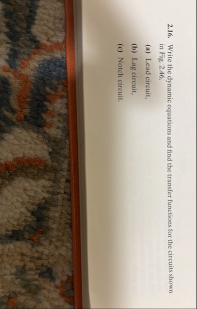
 BE.
~ NER
BRE CC
Ea 7
CAR 5
he
EE
E
This is AI generated Response.
Asked by: Alok Kumar
Created at: 2026-02-02 09:28:47
Asked by: Alok Kumar
Created at: 2026-02-02 09:28:47
Final Answer:
Rendered
Raw Text
Did you like this answer?
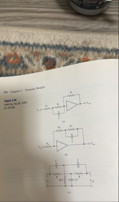
Absolutely! Let's go step by step for each circuit in **Figure 2.46**.
---
# 2.16: Write the dynamic equations and find the transfer functions
## (a) **Lead Circuit**
### **Circuit Description**
- Input: \( V_{in} \)
- Output: \( V_{out} \)
- Series: \( R_1 \) and \( C \)
- Feedback: \( R_f \) (Op-amp configuration)
#### **Dynamic Equation**
This is a **lead compensator** (high-pass RC in the feedback):
- The impedance of the RC network: \( Z_{RC} = R_1 + \frac{1}{sC} \)
- The transfer function (assuming ideal op-amp, inverting):
\[
V_{out} = -V_{in} \left( \frac{Z_f}{Z_{in}} \right)
\]
Where:
- \( Z_{in} = R_1 \)
- \( Z_f = \frac{R_f}{1 + sR_fC} \) (parallel combination of \( R_f \) and \( C \))
\[
H(s) = \frac{V_{out}}{V_{in}} = -\frac{Z_f}{Z_{in}}
\]
For the lead configuration, you typically get:
\[
H(s) = -\frac{R_f}{R_1} \cdot \frac{1 + sR_1C}{1 + sR_fC}
\]
---
## (b) **Lag Circuit**
### **Circuit Description**
- Input: \( V_{in} \)
- Output: \( V_{out} \)
- Series: \( R_1 \)
- Feedback: \( R_f \) and \( C \) (in parallel)
#### **Dynamic Equation**
This is a **lag compensator** (low-pass RC in the feedback):
- \( Z_{in} = R_1 + \frac{1}{sC} \)
- \( Z_f = R_f \)
\[
H(s) = -\frac{R_f}{R_1 + \frac{1}{sC}}
\]
\[
= -\frac{R_f sC}{1 + R_1 sC}
\]
But for the standard lag compensator, the transfer function is generally:
\[
H(s) = -\frac{R_f}{R_1} \cdot \frac{1 + sR_1C}{1 + sR_fC}
\]
But the configuration here is slightly different (feedback and input swap).
---
## (c) **Notch Circuit**
### **Circuit Description**
- Input: \( V_{in} \)
- Output: \( V_{out} \)
- Two capacitors in series, with a parallel branch of \( R \) and \( 2R \)
#### **Dynamic Equation**
This circuit is a **notch (band-stop) filter**.
- The transfer function for a standard notch filter:
\[
H(s) = \frac{s^2 + \omega_^2}{s^2 + \frac{\omega_}{Q}s + \omega_^2}
\]
For this specific configuration, you’d write the node equations (using KCL or voltage divider) to get the exact transfer function.
---
## **Summary Table**
| Circuit | Type | Transfer Function (standard form) |
|---------|--------|-----------------------------------------------|
| (a) | Lead | \( H(s) = -\frac{R_f}{R_1} \cdot \frac{1 + sR_1C}{1 + sR_fC} \) |
| (b) | Lag | \( H(s) = -\frac{R_f}{R_1} \cdot \frac{1 + sR_1C}{1 + sR_fC} \) (swap \( R_f, R_1 \)) |
| (c) | Notch | \( H(s) = \frac{s^2 + \omega_^2}{s^2 + \frac{\omega_}{Q}s + \omega_^2} \) |
---
## **Tips**
- For op-amp circuits, always use the formula: \( H(s) = -\frac{Z_f}{Z_{in}} \) for inverting configurations.
- For passive notch filters, use voltage divider principles and impedance algebra.
If you want the detailed step-by-step derivation for any one of these, let me know which one!
Question:
complete solution not in tabular format pls
This is AI generated Response.
Asked by: Alok Kumar
Created at: 2026-02-02 09:34:04
Asked by: Alok Kumar
Created at: 2026-02-02 09:34:04
Final Answer:
Rendered
Raw Text
Did you like this answer?
# Dynamic Equations and Transfer Functions
In this section, we will derive the dynamic equations and transfer functions for different types of circuits.
## 1. Lead Circuit
### Circuit Description
- **Input:** \( V_{in} \)
- **Output:** \( V_{out} \)
- **Components:**
- Resistor \( R_1 \)
- Capacitor \( C \)
- Feedback Resistor \( R_f \) (in an op-amp configuration)
### Dynamic Equation
The lead compensator typically acts as a high-pass filter in the feedback. The impedance of the RC network is given by:
\[
Z_{RC} = R_1 + \frac{1}{sC}
\]
The transfer function can be expressed as follows:
\[
H(s) = -\frac{Z_f}{Z_{in}}
\]
Where:
- \( Z_{in} = R_1 \)
- \( Z_f = \frac{R_f}{1 + sR_fC} \) (for the feedback path)
Thus, the overall transfer function is:
\[
H(s) = -\frac{R_f}{R_1} \cdot \frac{1 + sR_1C}{1 + sR_fC}
\]
---
## 2. Lag Circuit
### Circuit Description
- **Input:** \( V_{in} \)
- **Output:** \( V_{out} \)
- **Components:**
- Resistor \( R_1 \)
- Feedback Resistor \( R_f \)
- Capacitor \( C \)
### Dynamic Equation
The lag compensator acts as a low-pass filter. The impedance can be represented as:
\[
Z_{in} = R_1 + \frac{1}{sC}
\]
The feedback impedance is simply:
\[
Z_f = R_f
\]
The transfer function for this configuration is:
\[
H(s) = -\frac{R_f}{R_1 + \frac{1}{sC}} = -\frac{R_f sC}{1 + R_1 sC}
\]
The standard form for the lag compensator is:
\[
H(s) = -\frac{R_f}{R_1} \cdot \frac{1 + sR_1C}{1 + sR_fC}
\]
---
## 3. Notch Circuit
### Circuit Description
- **Input:** \( V_{in} \)
- **Output:** \( V_{out} \)
- **Components:**
- Two capacitors in series
- A resistor \( R \) and \( 2R \) in parallel
### Dynamic Equation
The notch filter is designed to eliminate specific frequency components. The transfer function can be expressed as:
\[
H(s) = \frac{s^2 + \omega_0^2}{s^2 + \frac{\omega_0}{Q}s + \omega_0^2}
\]
Where:
- \( \omega_0 \) is the resonant frequency
- \( Q \) is the quality factor
To derive the exact transfer function, apply Kirchhoff's current law (KCL) or use voltage divider principles.
---
## Summary
In summary, the transfer functions for the circuits are:
- **Lead Circuit:**
\[
H(s) = -\frac{R_f}{R_1} \cdot \frac{1 + sR_1C}{1 + sR_fC}
\]
- **Lag Circuit:**
\[
H(s) = -\frac{R_f}{R_1} \cdot \frac{1 + sR_1C}{1 + sR_fC}
\]
- **Notch Circuit:**
\[
H(s) = \frac{s^2 + \omega_0^2}{s^2 + \frac{\omega_0}{Q}s + \omega_0^2}
\]
These equations provide the necessary foundation for analyzing the behavior of each circuit type. If you require further clarification on any specific circuit or concept, feel free to ask!
Question:
Suppose an investment doubles in value over three years. What is the average annual simple return and the average annual log return?
This is AI generated Response.
Asked by: Alok Kumar
Created at: 2026-02-04 18:06:03
Asked by: Alok Kumar
Created at: 2026-02-04 18:06:03
Final Answer:
Rendered
Raw Text
Did you like this answer?
To calculate the average annual simple return and the average annual log return for an investment that doubles in value over three years, we can use the following formulas:
## 1. Average Annual Simple Return
### Formula
The simple return can be calculated using the formula:
\[
R = \frac{V_f - V_i}{V_i}
\]
Where:
- \( V_f \) = final value
- \( V_i \) = initial value
If the investment doubles, then \( V_f = 2V_i \).
### Calculation
Substituting into the formula:
\[
R = \frac{2V_i - V_i}{V_i} = \frac{V_i}{V_i} = 1
\]
The total return over three years is 100%, so the average annual simple return is:
\[
\text{Average Annual Simple Return} = \frac{R}{n} = \frac{1}{3} = 0.3333 \text{ or } 33.33\%
\]
---
## 2. Average Annual Log Return
### Formula
The log return can be calculated using the formula:
\[
r = \ln\left(\frac{V_f}{V_i}\right)
\]
### Calculation
For our case:
\[
r = \ln\left(\frac{2V_i}{V_i}\right) = \ln(2)
\]
Calculating \( \ln(2) \):
\[
r \approx 0.6931
\]
To find the average annual log return over three years:
\[
\text{Average Annual Log Return} = \frac{r}{n} = \frac{0.6931}{3} \approx 0.2310 \text{ or } 23.10\%
\]
---
## Summary
- **Average Annual Simple Return:** \( 33.33\% \)
- **Average Annual Log Return:** \( 23.10\% \)
These returns help assess the investment's performance over the specified period. If you have further questions about these calculations, feel free to ask!
Question:
Company ABC's stock has a beta of 1 . 2 , the risk - free rate is 4 % , and the expected market return is 1 0 % . According to the Capital Asset Pricing Model ( CAPM ) , what is the expected return on Company ABC's stock? Select one: 1 6 . 5 % 1 4 . 7 % 1 8 % 1 0 % 1 1 . 2 %
This is AI generated Response.
Asked by: Alok Kumar
Created at: 2026-02-04 18:25:55
Asked by: Alok Kumar
Created at: 2026-02-04 18:25:55
Final Answer:
Rendered
Raw Text
Did you like this answer?
To find the expected return on Company ABC's stock using the Capital Asset Pricing Model (CAPM), we can use the following formula:
## CAPM Formula
\[
E(R) = R_f + \beta \times (E(R_m) - R_f)
\]
Where:
- \( E(R) \) = expected return on the stock
- \( R_f \) = risk-free rate
- \( \beta \) = beta of the stock
- \( E(R_m) \) = expected market return
### Given Values
- \( \beta = 1.2 \)
- \( R_f = 4\% = 0.04 \)
- \( E(R_m) = 10\% = 0.10 \)
### Calculation Steps
1. Calculate the market risk premium:
\[
E(R_m) - R_f = 0.10 - 0.04 = 0.06
\]
2. Substitute the values into the CAPM formula:
\[
E(R) = 0.04 + 1.2 \times 0.06
\]
3. Perform the multiplication:
\[
1.2 \times 0.06 = 0.072
\]
4. Add to the risk-free rate:
\[
E(R) = 0.04 + 0.072 = 0.112
\]
5. Convert to percentage:
\[
E(R) = 0.112 \times 100 = 11.2\%
\]
---
## Conclusion
The expected return on Company ABC's stock according to the CAPM is **11.2%**.
### Answer:
**11.2%**
📢 Instructions:
- Ask anything relatd to above question only.
- For new Question goto :