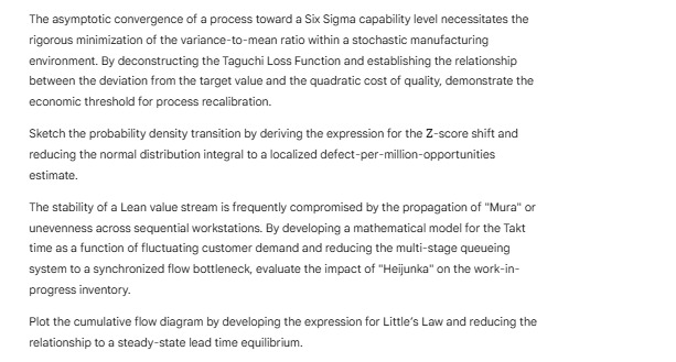
Act like a helpful tutor and exlain me :The asymptotic convergence of a process toward a Si Sigma capabilty level necessitates the
figorous minimization of the variance-to-mean ratio within a stochastic manufacturing
environment. By deconstructing the Taguchi Loss Function and establishing the relationship.
between the deviation from the target valus and the quadratic cost of quay, demonstrate the
economic threshold for process recalibration
‘Sketch the probability density transition by deriving the expression for the Z-score shift and
reducing the normal distribution integral to a localized defect-per-milfn-opportunities
estimate,
The stabity of a Lean value stream i frequently compromisad by the propagation of Mura" or
unevenness across sequential workstations. By developing a mathematical model for the Takt
time as: function of fluctuating customer demand and reducing the multi-stage queueing
system 10.2 synchronized flow bottienack, evaluate the impact of "Hefunka” on the work-in-
progress inventory.
Plot the cumulative flow diagram by developing the expression for Little's Law and reducing the
relationship to a steady-state lead time equilbrium.
Question:
Act like a helpful tutor and exlain me :The asymptotic convergence of a process toward a Si Sigma capabilty level necessitates the
figorous minimization of the variance-to-mean ratio within a stochastic manufacturing
environment. By deconstructing the Taguchi Loss Function and establishing the relationship.
between the deviation from the target valus and the quadratic cost of quay, demonstrate the
economic threshold for process recalibration
‘Sketch the probability density transition by deriving the expression for the Z-score shift and
reducing the normal distribution integral to a localized defect-per-milfn-opportunities
estimate,
The stabity of a Lean value stream i frequently compromisad by the propagation of Mura" or
unevenness across sequential workstations. By developing a mathematical model for the Takt
time as: function of fluctuating customer demand and reducing the multi-stage queueing
system 10.2 synchronized flow bottienack, evaluate the impact of "Hefunka” on the work-in-
progress inventory.
Plot the cumulative flow diagram by developing the expression for Little's Law and reducing the
relationship to a steady-state lead time equilbrium.
This is AI generated Response.
Asked by: Alok Kumar
Created at: 2026-01-31 09:04:11
Final Answer:
RenderedRaw Text
Did you like this answer?
Absolutely! Let me break down each paragraph into simpler explanations, step by step:
---
## 1. Six Sigma, Variance, and the Taguchi Loss Function
**Original:**
*The asymptotic convergence of a process toward a Six Sigma capability level necessitates the rigorous minimization of the variance-to-mean ratio within a stochastic manufacturing environment. By deconstructing the Taguchi Loss Function and establishing the relationship between the deviation from the target value and the quadratic cost of quality, demonstrate the economic threshold for process recalibration.*
**Explanation:**
- **Six Sigma capability:** Refers to a process that is extremely well controlled, with very few defects (3.4 per million opportunities).
- **Variance-to-mean ratio:** Measures how much variation there is in your process compared to the average output.
- **Taguchi Loss Function:** This is a formula that shows how the cost (or "loss") increases as your process output deviates from the target value. The loss increases **quadratically** (i.e., much faster as you move further from the target).
- **Economic threshold:** The point at which the cost of poor quality justifies recalibrating (fixing) the process.
**In short:**
Minimize process variation to approach Six Sigma quality. Use the Taguchi Loss Function to quantify how much deviation from the target costs you, and decide when it’s economically smart to recalibrate your process.
---
## 2. Z-Score, Normal Distribution, and DPMO
**Original:**
*Sketch the probability density transition by deriving the expression for the Z-score shift and reducing the normal distribution integral to a localized defect-per-million-opportunities estimate.*
**Explanation:**
- **Z-score:** Tells you how many standard deviations a value is from the mean.
- **Normal distribution:** The classic "bell curve" describing how data is distributed around the average.
- **Defects per million opportunities (DPMO):** A way to express process quality in Six Sigma, showing how many defects you’d expect if you had a million chances to make a mistake.
**In short:**
Calculate how shifting the Z-score (process mean relative to specification limits) changes the area under the normal curve beyond your specification limits, and convert this area to an expected number of defects per million.
---
## 3. Lean Value Stream, Mura, Takt Time, and Heijunka
**Original:**
*The stability of a Lean value stream is frequently compromised by the propagation of "Mura" or unevenness across sequential workstations. By developing a mathematical model for the Takt time as a function of fluctuating customer demand and reducing the multi-stage queueing system to a synchronized flow bottleneck, evaluate the impact of "Heijunka" on the work-in-progress inventory.*
**Explanation:**
- **Lean value stream:** The sequence of activities that add value to a product in Lean manufacturing.
- **Mura:** Japanese term for unevenness or inconsistency in production.
- **Takt time:** The pace of production needed to meet customer demand.
- **Heijunka:** Production leveling—smoothing out production to avoid peaks and valleys.
- **Work-in-progress (WIP) inventory:** Items that are being processed but not yet finished.
**In short:**
Uneven production causes problems. Use math to model how changing customer demand affects the pace of work (Takt time). By leveling production (Heijunka), you reduce bottlenecks and WIP inventory, making the flow more stable.
---
## 4. Little’s Law and Cumulative Flow
**Original:**
*Plot the cumulative flow diagram by developing the expression for Little’s Law and reducing the relationship to a steady-state lead time equilibrium.*
**Explanation:**
- **Little’s Law:** A fundamental queuing principle:
\[
\text{Average Inventory (WIP)} = \text{Arrival Rate} \times \text{Average Lead Time}
\]
- **Cumulative flow diagram:** A chart showing how tasks flow through different stages of a process over time.
- **Steady-state lead time:** The average time it takes for an item to go from start to finish when the system is in equilibrium (input rate = output rate).
**In short:**
Use Little’s Law to relate how many items are in the system to how fast they arrive and how long they stay. Plot how work items accumulate and move through the process, aiming for a stable, predictable flow.
---
**Let me know which concept you'd like to see an example or more math for!**
Question:
summary pls
This is AI generated Response.
Asked by: Alok Kumar
Created at: 2026-01-31 09:07:20
Final Answer:
RenderedRaw Text
Did you like this answer?
# Summary of Key Concepts in Manufacturing Processes
## 1. Six Sigma and Taguchi Loss Function
- **Six Sigma:** Aiming for minimal defects (3.4 per million).
- **Variance-to-Mean Ratio:** Important for process control.
- **Taguchi Loss Function:** Costs increase quadratically with deviation from target.
- **Economic Threshold:** Determine when recalibration is justified based on costs.
## 2. Z-Score and Defects Per Million Opportunities (DPMO)
- **Z-Score:** Measures how far a value is from the mean.
- **Normal Distribution:** Represents data around the average.
- **DPMO:** Expresses expected defects per million opportunities based on the Z-score shift.
## 3. Lean Value Stream and Heijunka
- **Lean Value Stream:** Sequence of activities adding value.
- **Mura:** Refers to unevenness in production.
- **Takt Time:** Production rate to meet customer demand.
- **Heijunka:** Leveling production to smooth out flow and reduce WIP inventory.
## 4. Little’s Law and Cumulative Flow
- **Little's Law:**
\[
\text{Average Inventory (WIP)} = \text{Arrival Rate} \times \text{Average Lead Time}
\]
- **Cumulative Flow Diagram:** Visualizes the flow of tasks through stages.
- **Steady-State Lead Time:** Average time for an item to complete the process in equilibrium.
---
This concise summary outlines the main concepts and relationships important for understanding quality control and efficiency in manufacturing processes. Let me know if you need further details on any specific topic!
VIPSolutions focuses on clear, step‑by‑step explanations so you can learn quickly. Whether you need an AI‑generated walkthrough or a short hint to get unstuck, each solution is organized for fast reading and easy review later.
Search similar questions, compare approaches, and bookmark the best answers for revision. Our goal is simple: quick, reliable study help that feels natural—not noisy.
 VIPSolutions
 The asymptotic convergence of a process toward a Si Sigma capabilty level necessitates the
figorous minimization of the variance-to-mean ratio within a stochastic manufacturing
environment. By deconstructing the Taguchi Loss Function and establishing the relationship.
between the deviation from the target valus and the quadratic cost of quay, demonstrate the
economic threshold for process recalibration
‘Sketch the probability density transition by deriving the expression for the Z-score shift and
reducing the normal distribution integral to a localized defect-per-milfn-opportunities
estimate,
The stabity of a Lean value stream i frequently compromisad by the propagation of Mura" or
unevenness across sequential workstations. By developing a mathematical model for the Takt
time as: function of fluctuating customer demand and reducing the multi-stage queueing
system 10.2 synchronized flow bottienack, evaluate the impact of "Hefunka” on the work-in-
progress inventory.
Plot the cumulative flow diagram by developing the expression for Little's Law and reducing the
relationship to a steady-state lead time equilbrium.