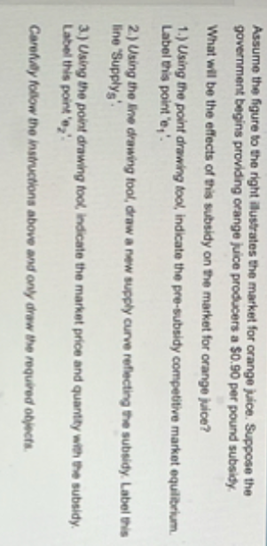
# Step-by-Step Solution: Market for Orange Juice (Microeconomics) ## **Micro or Macro?** This is a **microeconomic** question because it deals with the effects of a subsidy in a specific market (orange juice), not the whole economy. --- ## **Question Summary** A government gives orange juice producers a $.50 per pound subsidy. You are to: 1. Indicate the pre-subsidy equilibrium. 2. Draw the new supply curve with the subsidy. 3. Indicate the new equilibrium (price & quantity). --- ## **Step 1: Pre-Subsidy Equilibrium (Point E₁)** - **Find where the original supply and demand curves intersect.** - This is the **competitive market equilibrium** (before subsidy). - Label this point **E₁**. 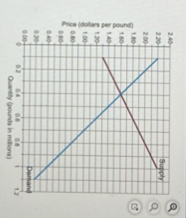**On the graph:** - Look for the intersection of the blue (Demand) and brown (Supply) lines. - The corresponding price and quantity are the pre-subsidy equilibrium. --- ## **Step 2: Draw the New Supply Curve (S')** - **A subsidy to producers shifts the supply curve down (right) by the amount of the subsidy ($.50).** - This means for every quantity, the new supply curve is $.50 lower in price than the original. - Draw a new supply curve parallel to the original, but $.50 lower at every point. - Label this new curve **S'**. --- ## **Step 3: New Equilibrium (Point E₂)** - **Find the intersection of the new supply curve (S') and the demand curve.** - This is the **new market equilibrium** (after subsidy). - Label this point **E₂**. **On the graph:** - Where S' (shifted supply) meets Demand is the new equilibrium. - The corresponding price (paid by consumers) is lower, and quantity is higher than before. --- ## **Summary Table** | Step | What to Do | How to Show on Graph | |------|------------|---------------------| | 1 | Indicate pre-subsidy equilibrium | Intersection of original Supply and Demand (label E₁) | | 2 | Draw new supply with subsidy | Shift original Supply curve down by $.50 (label S') | | 3 | Indicate new equilibrium | Intersection of Demand and S' (label E₂) | --- ## **Effects of the Subsidy** - **Price for consumers falls** - **Quantity sold increases** - **Producers receive the market price + $.50 subsidy per pound** --- ### **Graphical Illustration Steps (Text Based)** 1. **Mark E₁**: Find where the Demand and original Supply curve cross. 2. **Draw S'**: For each quantity, plot a point $.50 lower in price than the original supply, and connect these points. 3. **Mark E₂**: Find where Demand crosses S', and mark this as E₂. --- If you need a visual drawing or further calculation, let me know!

# Step-by-Step Solution: Analyzing the Impact of a Subsidy on Orange Juice Market ## **Micro or Macro?** This question pertains to **microeconomics** as it focuses on the impact of a subsidy on a specific market (orange juice), rather than the economy as a whole. --- ## **Problem Overview** The government provides a subsidy of $0.50 per pound to orange juice producers. You will: 1. Identify the pre-subsidy equilibrium. 2. Illustrate the new supply curve with the subsidy. 3. Determine the new market equilibrium (price and quantity). --- ## **Step 1: Pre-Subsidy Equilibrium (E₁)** - **Objective**: Locate the intersection of the original supply and demand curves. - This intersection represents the **pre-subsidy equilibrium**. **Instructions**: - On the graph, find the point where the original **Demand** (D) and **Supply** (S) curves intersect. - Label this point as **E₁**. --- ## **Step 2: Adjusting the Supply Curve (S')** - **Objective**: Shift the supply curve downwards by the amount of the subsidy ($0.50). - This adjustment reflects that producers can supply the same quantity at a lower price due to the subsidy. **Instructions**: - Draw a new supply curve, **S'**, parallel to the original supply curve (S), but positioned $0.50 lower at each quantity level. - This shift represents the increased willingness of producers to supply orange juice at a lower price. --- ## **Step 3: New Equilibrium (E₂)** - **Objective**: Identify the new equilibrium after the subsidy. - This is where the new supply curve (S') intersects the demand curve. **Instructions**: - On the graph, find the intersection point between the **Demand** curve and the new **Supply** curve (S'). - Label this new intersection as **E₂**. --- ## **Summary of Findings** | Step | Description | Graphical Representation | |------|-------------|--------------------------| | 1 | Identify pre-subsidy equilibrium | Intersection of original Supply (S) and Demand (D) at E₁ | | 2 | Adjust supply for subsidy | Draw new Supply curve (S') shifted down by $0.50 | | 3 | Determine new equilibrium | Intersection of Demand and new Supply (S') at E₂ | --- ## **Effects of the Subsidy** - **Consumer Price**: The price consumers pay for orange juice decreases. - **Quantity Sold**: The total quantity of orange juice sold in the market increases. - **Producer Revenue**: Producers benefit from the market price plus an additional $0.50 per pound from the subsidy. --- ### **Visual Representation Steps** 1. **Mark E₁**: Identify and label the intersection of the original demand and supply curves on the graph. 2. **Draw S'**: Shift the supply curve downwards by $0.50 for each quantity and label this new curve as S'. 3. **Mark E₂**: Identify the new equilibrium by finding the intersection of the demand and the new supply curve (S') and label it as E₂. --- If you need further clarifications or calculations, feel free to ask!

# Summary: Impact of a $0.50 Subsidy on the Orange Juice Market ## **Microeconomic Context** This analysis focuses on microeconomic principles by examining the effects of a government subsidy on the specific market for orange juice. --- ## **Key Concepts** 1. **Pre-Subsidy Equilibrium (E₁)**: - The initial intersection of the demand and original supply curves determines the price and quantity before any subsidy is provided. 2. **New Supply Curve with Subsidy (S')**: - A subsidy of $0.50 lowers the cost for producers, shifting the supply curve downward (rightward) by the subsidy amount. - The new supply curve (S') is parallel to the original supply curve, indicating that producers can supply the same quantity at a lower price. 3. **Post-Subsidy Equilibrium (E₂)**: - The new equilibrium is found at the intersection of the demand curve and the shifted supply curve (S'). - The price paid by consumers decreases, and the quantity sold in the market increases due to the subsidy. --- ## **Graphical Illustration** - **E₁**: Original equilibrium point where demand intersects the original supply curve. - **S'**: New supply curve reflecting the $0.50 subsidy. - **E₂**: New equilibrium point where demand intersects the shifted supply curve. --- ## **Effects of the Subsidy** - **Consumer Benefits**: Lower prices for orange juice. - **Increased Quantity**: Higher quantity sold in the market. - **Producer Gains**: Producers receive a market price plus the $0.50 subsidy per pound. This summary encapsulates the shifts in supply and equilibrium in the orange juice market resulting from the subsidy, illustrating fundamental microeconomic principles.