 VIPSolutions
Give step-by-step solution with explanation and final answer:The Estimation of a Cobb-Douglas Production Function for China. Comin the Cob Dongs produto non y= aes JE Er E——— A TSI PEO Tout cn ee I Er I oh on qe th eget bps ci fi © Ee mum scat we hr preocn aco. ee sntrs Tot pt ee egw er th aa a aio ee ae Le te ey Le eis wk rar NT cet a. ths me thro as hem ee ees spilt rp eyed ye fo sh Bc
Question:
Give step-by-step solution with explanation and final answer: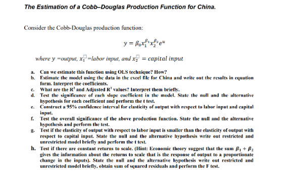 The Estimation of a Cobb-Douglas Production Function for China.
Comin the Cob Dongs produto non
y= aes
JE Er E———
A
TSI PEO Tout cn
ee
I Er
I oh on
qe th eget bps ci
fi
© Ee mum scat we hr preocn aco. ee sntrs
Tot pt
ee egw er th aa a aio
ee ae Le te ey Le
eis wk rar
NT cet a. ths me thro as hem
ee ees spilt
rp eyed
ye fo sh Bc
This is AI generated Response.
Asked by: Vikram Kumar
Created at: 2025-10-21 03:17:30
Asked by: Vikram Kumar
Created at: 2025-10-21 03:17:30
Final Answer:
Rendered
Raw Text
Did you like this answer?
Certainly! Here's a step-by-step guide to solving the problem related to the Cobb-Douglas production function for China.
---
# Step-by-step Solution for Estimating the Cobb-Douglas Production Function
## 1. **Understanding the Model**
The Cobb-Douglas production function is given by:
\[
y = \beta_ x_1^{\beta_1} x_2^{\beta_2} e^{u}
\]
- \( y \): Output
- \( x_1 \): Labor input
- \( x_2 \): Capital input
- \( \beta_ \): Constant term
- \( \beta_1, \beta_2 \): Elasticities of output with respect to labor and capital
- \( u \): Error term
---
## 2. **Transforming the Model for Estimation (OLS Technique)**
To estimate coefficients using Ordinary Least Squares (OLS), take the natural logarithm on both sides:
\[
\ln y = \ln \beta_ + \beta_1 \ln x_1 + \beta_2 \ln x_2 + u
\]
Define:
- \( Y = \ln y \)
- \( X_1 = \ln x_1 \)
- \( X_2 = \ln x_2 \)
- \( \alpha_ = \ln \beta_ \)
The linear form becomes:
\[
Y = \alpha_ + \beta_1 X_1 + \beta_2 X_2 + u
\]
---
## 3. **Estimate the Model Using Data**
- Collect data on \( y \), \( x_1 \), \( x_2 \).
- Calculate \( \ln y \), \( \ln x_1 \), \( \ln x_2 \).
- Run OLS regression of \( Y \) on \( X_1 \) and \( X_2 \).
---
## 4. **Interpreting the Results**
- **Coefficients \( \hat{\beta}_1 \), \( \hat{\beta}_2 \)**: Elasticities of output with respect to labor and capital.
- **Intercept \( \hat{\alpha}_ \)**: Log of \( \beta_ \), so exponentiate to get \( \hat{\beta}_ \).
---
## 5. **Hypotheses Testing**
- **Null hypothesis for each coefficient**: \( H_: \beta_i = \)
- **Alternative hypothesis**: \( H_A: \beta_i \neq \)
- Use t-statistics and p-values to test significance.
---
## 6. **Confidence Intervals**
Construct 95% confidence interval for each coefficient:
\[
\hat{\beta}_i \pm 1.96 \times \text{Standard Error}(\hat{\beta}_i)
\]
---
## 7. **Model Validity & Tests**
- **F-test**: Overall significance of the model.
- **R-squared**: Variance explained by the model.
- **Residual analysis**: Check for heteroskedasticity, autocorrelation, etc.
---
## 8. **Elasticity Interpretation**
- The estimated \( \hat{\beta}_1 \) indicates the percentage change in output for a 1% change in labor.
- The estimated \( \hat{\beta}_2 \) indicates the percentage change in output for a 1% change in capital.
---
## 9. **Final Equation**
After estimating, the model might look like:
\[
\hat{y} = \hat{\beta}_ \times x_1^{\hat{\beta}_1} \times x_2^{\hat{\beta}_2}
\]
where the parameters are from the regression output.
---
# Summary:
- Use the log-linear form for estimation via OLS.
- Interpret coefficients as elasticities.
- Test significance and construct confidence intervals.
- Validate the model assumptions before final inference.
---
If you provide data, I can guide through the actual calculations!
Question:
step by step answer provide ok
This is AI generated Response.
Asked by: Vikram Kumar
Created at: 2025-10-21 03:21:48
Asked by: Vikram Kumar
Created at: 2025-10-21 03:21:48
Final Answer:
Rendered
Raw Text
Did you like this answer?
# Step-by-Step Solution for Estimating the Cobb-Douglas Production Function
## 1. **Understanding the Cobb-Douglas Function**
The Cobb-Douglas production function is represented as:
\[
y = \beta_0 x_1^{\beta_1} x_2^{\beta_2} e^{u}
\]
Where:
- \( y \): Total output
- \( x_1 \): Labor input
- \( x_2 \): Capital input
- \( \beta_0 \): Constant term
- \( \beta_1, \beta_2 \): Output elasticities of labor and capital
- \( u \): Error term
---
## 2. **Logarithmic Transformation**
To convert this multiplicative function into a linear form suitable for estimation, take the natural logarithm:
\[
\ln y = \ln \beta_0 + \beta_1 \ln x_1 + \beta_2 \ln x_2 + u
\]
Define:
- \( Y = \ln y \)
- \( X_1 = \ln x_1 \)
- \( X_2 = \ln x_2 \)
- \( \alpha = \ln \beta_0 \)
The equation simplifies to:
\[
Y = \alpha + \beta_1 X_1 + \beta_2 X_2 + u
\]
---
## 3. **Data Collection**
Gather data on:
- Output (\( y \))
- Labor input (\( x_1 \))
- Capital input (\( x_2 \))
---
## 4. **Calculate Logarithms**
Compute the natural logarithms for the collected data:
\[
Y = \ln y, \quad X_1 = \ln x_1, \quad X_2 = \ln x_2
\]
---
## 5. **Run OLS Regression**
Perform Ordinary Least Squares (OLS) regression of \( Y \) on \( X_1 \) and \( X_2 \):
- Obtain estimates for \( \hat{\alpha} \), \( \hat{\beta}_1 \), and \( \hat{\beta}_2 \).
---
## 6. **Interpret the Results**
- **Coefficients \( \hat{\beta}_1 \) and \( \hat{\beta}_2 \)** show the elasticity of output with respect to labor and capital, respectively.
- **Intercept \( \hat{\alpha} \)** represents \( \ln \beta_0 \); exponentiate to find \( \hat{\beta_0} = e^{\hat{\alpha}} \).
---
## 7. **Hypothesis Testing**
Test the significance of each coefficient:
- **Null Hypothesis**: \( H_0: \beta_i = 0 \)
- **Alternative Hypothesis**: \( H_A: \beta_i \neq 0 \)
Use t-statistics and corresponding p-values for inference.
---
## 8. **Confidence Intervals**
Construct 95% confidence intervals for each coefficient:
\[
\hat{\beta}_i \pm 1.96 \times \text{Standard Error}(\hat{\beta}_i)
\]
---
## 9. **Model Validation**
Evaluate model fit and assumptions:
- **F-test**: Overall model significance.
- **R-squared**: Proportion of variance explained.
- **Residual analysis**: Check for assumptions like homoscedasticity and no autocorrelation.
---
## 10. **Final Production Function**
After the estimation process, the Cobb-Douglas production function can be represented as:
\[
\hat{y} = \hat{\beta}_0 \times x_1^{\hat{\beta}_1} \times x_2^{\hat{\beta}_2}
\]
---
# Summary
- Transform the Cobb-Douglas function into a linear model using logarithms.
- Collect and process the relevant data.
- Estimate parameters using OLS, interpret results, and validate the model.
- This provides a framework for understanding production dynamics in the context of labor and capital inputs.
📢 Instructions:
- Ask anything relatd to above question only.
- For new Question goto :