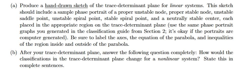
give answer in 2 step with explanation at the end of each step and final answer at the end:(a) Produce a hand-drawn sketch of the trace-determinant plane for linear systems. This sketch
should include a sample phase portrait of a proper unstable node, proper stable node, unstable
saddle point, unstable spiral point, stable spiral point, and a neutrally stable center, cach
placed in the appropriate region on the trace-determinant plane (use the same phase portrait
graphs you generated in the classification guide from Section 2; it’s okay if the portraits arc
computer generated). Be sure to label the axes, the equation of the parabola, and inequalities
of the region inside and outside of the parabola.
(b) After your trace-determinant plane, answer the following question completely: How would the
classifications in the trace-determinant plane change for a nonlinear system? State this in
complete sentences.
Question:
give answer in 2 step with explanation at the end of each step and final answer at the end:(a) Produce a hand-drawn sketch of the trace-determinant plane for linear systems. This sketch
should include a sample phase portrait of a proper unstable node, proper stable node, unstable
saddle point, unstable spiral point, stable spiral point, and a neutrally stable center, cach
placed in the appropriate region on the trace-determinant plane (use the same phase portrait
graphs you generated in the classification guide from Section 2; it’s okay if the portraits arc
computer generated). Be sure to label the axes, the equation of the parabola, and inequalities
of the region inside and outside of the parabola.
(b) After your trace-determinant plane, answer the following question completely: How would the
classifications in the trace-determinant plane change for a nonlinear system? State this in
complete sentences.
This is AI generated Response.
Asked by: Pagal
Created at: 2025-06-16 23:52:33
Final Answer:
RenderedRaw Text
Did you like this answer?
Sure! Let's break this into two clear steps as requested:
---
### **Step 1: Sketch and Explanation of the Trace-Determinant Plane for Linear Systems**
**Explanation:**
1. **Draw Axes & Parabola:**
- Draw a Cartesian plane with the **x-axis labeled as "Trace" (Tr)** and the **y-axis labeled as "Determinant" (Det)**.
- Draw the parabola given by the equation: **Det = (Tr/2)^2**, or equivalently, **Tr^2 = 4Det**. This parabola separates different types of equilibrium points.
2. **Label Regions and Place Sample Portraits:**
- **Above the parabola (Det > (Tr/2)^2, Det > 0):**
- If Tr > 0: Unstable spiral point (spiral source)
- If Tr < 0: Stable spiral point (spiral sink)
- **On the parabola (Det > 0, Tr^2 = 4Det):**
- If Tr > 0: Proper unstable node
- If Tr < 0: Proper stable node
- **Below the parabola (Det > 0, Tr^2 < 4Det):**
- Neutrally stable center (Tr = 0)
- **For Det < 0 (below the x-axis):**
- Saddle point (unstable)
- **Sample phase portraits** (small sketches) should be placed at each of these regions.
**Summary of placements:**
- **Saddle point**: Det < 0
- **Stable node**: Tr < 0, Det > 0, Tr^2 > 4Det
- **Unstable node**: Tr > 0, Det > 0, Tr^2 > 4Det
- **Stable spiral**: Tr < 0, Det > 0, Tr^2 < 4Det
- **Unstable spiral**: Tr > 0, Det > 0, Tr^2 < 4Det
- **Center**: Tr = 0, Det > 0, Tr^2 < 4Det
**Explanation at end of step:**
The trace-determinant plane helps us classify the stability and type of critical points for linear systems based on the values of the trace and determinant of the system's matrix. The shape and location relative to the parabola determine the nature of each equilibrium.
---
### **Step 2: Nonlinear Systems Classification**
**Explanation:**
For nonlinear systems, the classifications determined by the trace-determinant plane for linear systems do not always apply globally. The trace-determinant plane is strictly valid for linear systems or for analyzing the behavior near equilibrium points using the linearization (Jacobian matrix) of a nonlinear system. However, nonlinear systems can exhibit more complex behaviors such as limit cycles, bifurcations, and chaos, which are not captured by the linear trace-determinant classification. Additionally, the stability indicated by the linearization may not always reflect the true stability of the nonlinear system near the equilibrium, especially if the equilibrium is non-hyperbolic.
**Explanation at end of step:**
In summary, for nonlinear systems, the trace-determinant plane can only be used to infer local behavior near equilibrium points, and global dynamics may differ significantly from the linear case due to nonlinear effects.
---
### **Final Answer:**
1. **For linear systems**, the trace-determinant plane divides the trace-determinant space into regions corresponding to different types of equilibrium points (nodes, saddles, spirals, and centers), and sample phase portraits can be drawn in each region to illustrate the corresponding dynamical behavior.
2. **For nonlinear systems**, the trace-determinant classification only applies locally near equilibria and does not capture global behaviors unique to nonlinear systems, such as limit cycles or chaos. Nonlinearities can also cause the true stability to differ from that predicted by the linearization.
Question:
Solving a,b.
This is AI generated Response.
Asked by: Pagal
Created at: 2025-06-16 23:53:17
Final Answer:
RenderedRaw Text
Did you like this answer?
Certainly! Here's a detailed two-step explanation and solution for parts (a) and (b):
---
### **Step 1: Sketch and Explanation of the Trace-Determinant Plane for Linear Systems**
**Explanation:**
- **Axes and Parabola:**
- Draw a coordinate plane with **Trace (Tr)** on the x-axis and **Determinant (Det)** on the y-axis.
- The key curve is the parabola **Det = (Tr/2)^2** (or equivalently, **Tr² = 4Det**). This parabola separates regions with different stability characteristics.
- **Regions and Corresponding Dynamics:**
1. **Region outside the parabola with Det > 0:**
- **Tr > 0:**
- Tr > 0 and Tr² > 4Det → **Unstable node** (proper unstable node).
- **Sample portrait:** outward-spreading trajectories from the equilibrium.
- **Tr < 0:**
- Tr < 0 and Tr² > 4Det → **Stable node** (proper stable node).
- **Sample portrait:** trajectories converge into the equilibrium point.
2. **On the parabola with Det > 0:**
- **Tr > 0:**
- **Proper unstable node** (degenerate case).
- **Tr < 0:**
- **Proper stable node**.
3. **Inside the parabola (Tr² < 4Det, Det > 0):**
- **Tr = 0:**
- **Center (neutrally stable)** — trajectories are closed orbits.
- **Tr ≠ 0:**
- **Unstable spiral** if Tr > 0, or **Stable spiral** if Tr < 0.
- **Sample portraits:** spiral trajectories either inward or outward.
4. **Below the x-axis (Det < 0):**
- **Saddle point** — trajectories approach along one eigenvector and diverge along another.
- **Sample portrait:** saddle structure with hyperbolic trajectories.
**Summary:**
- The parabola **Det = (Tr/2)^2** acts as the boundary.
- Regions:
- **Det < 0:** saddle points.
- **Det > 0 and outside parabola:** nodes or spirals (stable/unstable).
- **Det > 0 and inside parabola:** centers or spirals.
- **Det > 0 and on parabola:** degenerate nodes.
*Label axes, parabola equation, and inequalities inside/outside regions accordingly.*
---
### **Step 2: Effect of Nonlinearities on Classifications**
**Explanation:**
In nonlinear systems, the trace-determinant classification derived from the linearization applies only **locally** near the equilibrium point. This is because the Jacobian matrix at the equilibrium determines the linear approximation, which indicates the local behavior. However:
- **Global behavior** can differ significantly: nonlinear terms can create phenomena like limit cycles, bifurcations, or chaos.
- **Stability** predicted by the linearization (via trace and determinant) may **not** reflect the true stability if the equilibrium is **non-hyperbolic** (eigenvalues with zero real part).
- **Bifurcations** may occur when parameters change, causing the system to transition between different types of behavior, often crossing the parabola boundary in the linear classification.
**Summary:**
In essence, the trace-determinant plane provides a **local** classification based on linear approximation. For nonlinear systems, these classifications are valid only in a small neighborhood around equilibrium points, and the **global dynamics** may involve behaviors not predictable solely from the linear analysis.
---
### **Final Answer:**
1. **The trace-determinant plane, with the parabola Det = (Tr/2)², partitions the space into regions corresponding to different types of equilibria (nodes, saddles, spirals, centers). Sample phase portraits placed in each region illustrate the local behavior of linear systems.**
2. **In nonlinear systems, the classifications based on trace and determinant apply only locally near equilibrium points. Nonlinearities can lead to phenomena like limit cycles or bifurcations, meaning the global dynamics may differ significantly from what the linear classification suggests.**
VIPSolutions focuses on clear, step‑by‑step explanations so you can learn quickly. Whether you need an AI‑generated walkthrough or a short hint to get unstuck, each solution is organized for fast reading and easy review later.
Search similar questions, compare approaches, and bookmark the best answers for revision. Our goal is simple: quick, reliable study help that feels natural—not noisy.
 VIPSolutions
 (a) Produce a hand-drawn sketch of the trace-determinant plane for linear systems. This sketch
should include a sample phase portrait of a proper unstable node, proper stable node, unstable
saddle point, unstable spiral point, stable spiral point, and a neutrally stable center, cach
placed in the appropriate region on the trace-determinant plane (use the same phase portrait
graphs you generated in the classification guide from Section 2; it’s okay if the portraits arc
computer generated). Be sure to label the axes, the equation of the parabola, and inequalities
of the region inside and outside of the parabola.
(b) After your trace-determinant plane, answer the following question completely: How would the
classifications in the trace-determinant plane change for a nonlinear system? State this in
complete sentences.