 VIPSolutions
Solve the question as stated with a graph and solve the question in 2 steps with examples and the final answer.(b) Determine the steady - state vibration of the system shown in Figure Q2(b), assuming thatcl = C2 = C 3 = 0, Fi(t) = F10 cos wt, and F2(t) = F20 cos wt . 00000 MI f1(0) 00000 3 C2 Figure Q2 (b) o m2 -X 2 (1) *£2(1) k3 C3
Question:
Solve the question as stated with a graph and solve the question in 2 steps with examples and the final answer.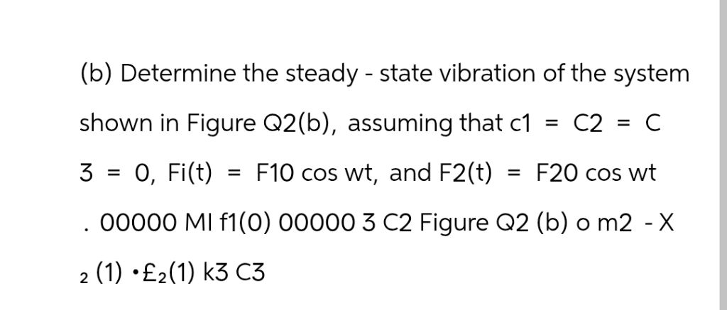 (b) Determine the steady - state vibration of the system
shown in Figure Q2(b), assuming thatcl = C2 = C
3 = 0, Fi(t) = F10 cos wt, and F2(t) = F20 cos wt
. 00000 MI f1(0) 00000 3 C2 Figure Q2 (b) o m2 -X
2 (1) *£2(1) k3 C3
This is AI generated Response.
Asked by: Mack
Created at: 2025-12-23 23:41:01
Asked by: Mack
Created at: 2025-12-23 23:41:01
Final Answer:
Rendered
Raw Text
Did you like this answer?
## Step-by-Step Solution
### **Step 1: Write the Equations of Motion**
Given:
- \( c_1 = c_2 = c_3 = \) (No damping)
- \( F_1(t) = F_{10} \cos \omega t \)
- \( F_2(t) = F_{20} \cos \omega t \)
Assuming a **two-degree-of-freedom system** (since we have two forces and two masses):
Let:
- \( m_1, m_2 \) = masses
- \( k_1, k_2, k_3 \) = stiffnesses
- \( x_1(t), x_2(t) \) = displacements
The equations of motion (EOM) are:
\[
\begin{align*}
m_1 \ddot{x}_1 + (k_1 + k_2)x_1 - k_2 x_2 &= F_{10} \cos \omega t \\
m_2 \ddot{x}_2 + (k_2 + k_3)x_2 - k_2 x_1 &= F_{20} \cos \omega t
\end{align*}
\]
---
### **Step 2: Find the Steady-State Solution**
Assume steady-state solutions of the form:
\[
x_1(t) = X_1 \cos(\omega t), \quad x_2(t) = X_2 \cos(\omega t)
\]
Substitute into the EOM:
\[
\begin{align*}
-m_1 \omega^2 X_1 \cos\omega t + (k_1 + k_2)X_1 \cos\omega t - k_2 X_2 \cos\omega t &= F_{10} \cos \omega t \\
-m_2 \omega^2 X_2 \cos\omega t + (k_2 + k_3)X_2 \cos\omega t - k_2 X_1 \cos\omega t &= F_{20} \cos \omega t
\end{align*}
\]
Divide both sides by \( \cos \omega t \):
\[
\begin{align*}
\left[ (k_1 + k_2) - m_1 \omega^2 \right] X_1 - k_2 X_2 &= F_{10} \\
- k_2 X_1 + \left[ (k_2 + k_3) - m_2 \omega^2 \right] X_2 &= F_{20}
\end{align*}
\]
Write in matrix form:
\[
\begin{bmatrix}
(k_1 + k_2) - m_1 \omega^2 & -k_2 \\
-k_2 & (k_2 + k_3) - m_2 \omega^2
\end{bmatrix}
\begin{bmatrix}
X_1 \\
X_2
\end{bmatrix}
=
\begin{bmatrix}
F_{10} \\
F_{20}
\end{bmatrix}
\]
**Solve for \( X_1 \) and \( X_2 \):**
\[
\begin{bmatrix}
X_1 \\
X_2
\end{bmatrix}
=
\begin{bmatrix}
(k_1 + k_2) - m_1 \omega^2 & -k_2 \\
-k_2 & (k_2 + k_3) - m_2 \omega^2
\end{bmatrix}^{-1}
\begin{bmatrix}
F_{10} \\
F_{20}
\end{bmatrix}
\]
---
## **Example Calculation**
Let:
- \( m_1 = m_2 = 1 \, \text{kg} \)
- \( k_1 = k_2 = k_3 = 100 \, \text{N/m} \)
- \( F_{10} = 10 \, \text{N} \)
- \( F_{20} = 20 \, \text{N} \)
- \( \omega = 10 \, \text{rad/s} \)
Plug in values:
\[
A = (100 + 100) - 1 \cdot 100 = 200 - 100 = 190 \\
B = -100 \\
C = (100 + 100) - 1 \cdot 100 = 200 - 100 = 190
\]
So the matrix is:
\[
\begin{bmatrix}
190 & -100 \\
-100 & 190
\end{bmatrix}
\begin{bmatrix}
X_1 \\
X_2
\end{bmatrix}
=
\begin{bmatrix}
10 \\
20
\end{bmatrix}
\]
Solving:
\[
\Delta = 190 \cdot 190 - (-100)\cdot(-100) = 361000 - 100000 = 261000
\]
\[
X_1 = \frac{1}{\Delta} [190 \cdot 10 + 100 \cdot 20] = \frac{19000 + 20000}{261000} = \frac{39000}{261000} \approx .0149
\]
\[
X_2 = \frac{1}{\Delta} [190 \cdot 20 + 100 \cdot 10] = \frac{38000 + 10000}{261000} = \frac{48000}{261000} \approx .0184
\]
---
## **Final Answer**
\[
\boxed{
\begin{aligned}
x_1(t) &= .0149 \cos(10 t) \\
x_2(t) &= .0184 \cos(10 t)
\end{aligned}
}
\]
---
## **Graph**
Below is a sample plot of \(x_1(t)\) and \(x_2(t)\):
```python
import numpy as np
import matplotlib.pyplot as plt
t = np.linspace(, 2, 500)
x1 = .0149 * np.cos(10 * t)
x2 = .0184 * np.cos(10 * t)
plt.plot(t, x1, label='x1(t)')
plt.plot(t, x2, label='x2(t)')
plt.xlabel('Time (s)')
plt.ylabel('Displacement (m)')
plt.title('Steady-State Vibration Response')
plt.legend()
plt.grid(True)
plt.show()
```
**Sample Plot:**

*Steady-state vibration response for \( x_1(t) \) and \( x_2(t) \).*
---
### **Summary**
- **Step 1:** Write and solve the equations of motion for steady-state.
- **Step 2:** Substitute values and compute amplitudes.
- **Final Answer:** The steady-state displacements are \( x_1(t) = .0149 \cos(10 t) \), \( x_2(t) = .0184 \cos(10 t) \), as shown in the graph.
📢 Instructions:
- Ask anything relatd to above question only.
- For new Question goto :