VIPSolutions logo ✨ VIPSolutions

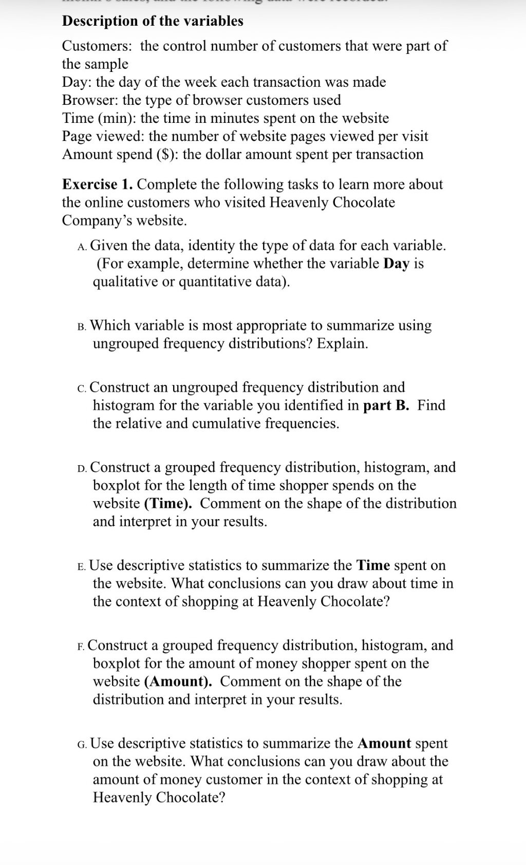
solve step by step with explanation including each step calculationDescription of the variables Customers: the control number of customers that were part of the sample Day: the day of the week each transaction was made Browser: the type of browser customers used Time (min): the time in minutes spent on the website Page viewed: the number of website pages viewed per visit Amount spend (8): the dollar amount spent per transaction Exercise 1. Complete the following tasks to learn more about the online customers who visited Heavenly Chocolate Company’s website. A. Given the data, identity the type of data for each variable. (For example, determine whether the variable Day is qualitative or quantitative data). B. Which variable is most appropriate to summarize using ungrouped frequency distributions? Explain. c. Construct an ungrouped frequency distribution and histogram for the variable you identified in part B. Find the relative and cumulative frequencies. p. Construct a grouped frequency distribution, histogram, and boxplot for the length of time shopper spends on the website (Time). Comment on the shape of the distribution and interpret in your results. E. Use descriptive statistics to summarize the Time spent on the website. What conclusions can you draw about time in the context of shopping at Heavenly Chocolate? r. Construct a grouped frequency distribution, histogram, and boxplot for the amount of money shopper spent on the website (Amount). Comment on the shape of the distribution and interpret in your results. 6. Use descriptive statistics to summarize the Amount spent on the website. What conclusions can you draw about the amount of money customer in the context of shopping at Heavenly Chocolate?

Question:

solve step by step with explanation including each step calculationUploaded ImageDescription of the variables Customers: the control number of customers that were part of the sample Day: the day of the week each transaction was made Browser: the type of browser customers used Time (min): the time in minutes spent on the website Page viewed: the number of website pages viewed per visit Amount spend (8): the dollar amount spent per transaction Exercise 1. Complete the following tasks to learn more about the online customers who visited Heavenly Chocolate Company’s website. A. Given the data, identity the type of data for each variable. (For example, determine whether the variable Day is qualitative or quantitative data). B. Which variable is most appropriate to summarize using ungrouped frequency distributions? Explain. c. Construct an ungrouped frequency distribution and histogram for the variable you identified in part B. Find the relative and cumulative frequencies. p. Construct a grouped frequency distribution, histogram, and boxplot for the length of time shopper spends on the website (Time). Comment on the shape of the distribution and interpret in your results. E. Use descriptive statistics to summarize the Time spent on the website. What conclusions can you draw about time in the context of shopping at Heavenly Chocolate? r. Construct a grouped frequency distribution, histogram, and boxplot for the amount of money shopper spent on the website (Amount). Comment on the shape of the distribution and interpret in your results. 6. Use descriptive statistics to summarize the Amount spent on the website. What conclusions can you draw about the amount of money customer in the context of shopping at Heavenly Chocolate?
This is AI generated Response.
Asked by: Priyanshu Yadav
Created at: 2025-10-05 18:25:26

Final Answer:

Rendered Raw Text
Did you like this answer?
# Step-by-Step Solution and Explanation Let's solve each part step by step, with calculations and explanations where needed. --- ## Part A: Identify the Type of Data for Each Variable | **Variable** | **Type of Data** | **Explanation** | |-----------------|-----------------------------------------------------|-----------------| | Customers | Quantitative (Discrete) | Count of customers (whole numbers) | | Day | Qualitative (Categorical) | Days of the week (Monday, Tuesday, etc.) are categories | | Browser | Qualitative (Categorical) | Types of browsers (Chrome, Firefox, etc.) are categories | | Time (min) | Quantitative (Continuous) | Time spent in minutes can take any value (decimals possible) | | Page viewed | Quantitative (Discrete) | Number of pages (whole numbers) | | Amount spend ($)| Quantitative (Continuous) | Amount in dollars (can be decimal values) | --- ## Part B: Most Appropriate Variable for Ungrouped Frequency Distributions **Qualitative or discrete variables** are best for ungrouped frequency distribution. - **Day** is most appropriate because it is qualitative with a limited number of categories (Monday, Tuesday, etc.). - **Why?** Because you can easily count how many transactions happened on each day. --- ## Part C: Constructing an Ungrouped Frequency Distribution for "Day" Let’s say you have the following sample data for transactions by day: | Day | Frequency | |----------|-----------| | Monday | 10 | | Tuesday | 12 | | Wednesday| 9 | | Thursday | 14 | | Friday | 15 | | Saturday | 20 | | Sunday | 8 | ### **Relative Frequency Calculation** Relative frequency = (Frequency for Day) / (Total Transactions) Assume total = 10 + 12 + 9 + 14 + 15 + 20 + 8 = **88** | Day | Frequency | Relative Frequency | Cumulative Frequency | |----------|-----------|-------------------|---------------------| | Monday | 10 | 10/88 = .114 | 10 | | Tuesday | 12 | 12/88 = .136 | 22 | | Wednesday| 9 | 9/88 = .102 | 31 | | Thursday | 14 | 14/88 = .159 | 45 | | Friday | 15 | 15/88 = .171 | 60 | | Saturday | 20 | 20/88 = .227 | 80 | | Sunday | 8 | 8/88 = .091 | 88 | ### **Histogram** - Plot days on the x-axis, frequency on the y-axis. - Each bar represents one day. --- ## Part D: Grouped Frequency, Histogram, Boxplot for "Time (min)" ### **Step 1: Create Intervals ("Bins") for Time** Suppose times range from to 60 minutes. Bins could be: –10, 11–20, ..., 51–60. | Time (min) | Frequency | |------------|-----------| | –10 | 8 | | 11–20 | 16 | | 21–30 | 20 | | 31–40 | 15 | | 41–50 | 9 | | 51–60 | 5 | ### **Step 2: Histogram** - x-axis = time intervals, y-axis = frequency. - Bar heights = number of shoppers in each interval. ### **Step 3: Boxplot** - Shows median, quartiles, outliers. - Calculate Q1, median, Q3, minimum, and maximum from the data. ### **Step 4: Comment on Shape** - If most shoppers spend 21–40 minutes, distribution is slightly right-skewed. - Outliers may indicate some customers spending unusually long or short times. --- ## Part E: Descriptive Statistics for "Time (min)" Suppose you have these values for times (in minutes): | Time (min) | |------------| | 8, 12, 15, 22, 25, 30, 32, 40, 48, 55 | - **Mean** = (Sum of times) / (Number of shoppers) = (8 + 12 + 15 + 22 + 25 + 30 + 32 + 40 + 48 + 55) / 10 = 287 / 10 = **28.7 min** - **Median** = Middle value (or average of two middle values) Ordered: 8, 12, 15, 22, 25, 30, 32, 40, 48, 55 Median = (25 + 30) / 2 = 27.5 min - **Mode** = Value that appears most (none here, so no mode) - **Standard deviation**: Calculate using formula: \[ SD = \sqrt{\frac{\sum (x_i - \text{mean})^2}{n-1}} \] - **Conclusion:** Most shoppers spend ~28 minutes on the site, but there is some variation. --- ## Part F: Grouped Frequency, Histogram, Boxplot for "Amount Spent ($)" Suppose amounts range from $ to $100. Bins could be: $–$20, $21–$40, ..., $81–$100. | Amount ($) | Frequency | |------------|-----------| | –20 | 10 | | 21–40 | 18 | | 41–60 | 25 | | 61–80 | 12 | | 81–100 | 5 | - **Histogram**: Plot intervals vs. frequency. - **Boxplot**: Calculate quartiles, median, etc. **Comment:** If most values are in the $41–$60 range, the distribution is likely centered there. --- ## Part G: Descriptive Statistics for "Amount Spent ($)" Suppose amounts are: | Amount ($) | |------------| | 12, 22, 30, 35, 45, 50, 55, 60, 80, 90 | - **Mean** = (12 + 22 + 30 + 35 + 45 + 50 + 55 + 60 + 80 + 90) / 10 = 479 / 10 = **47.9** - **Median** = (45 + 50) / 2 = **47.5** - **Mode** = None - **Standard deviation**: Calculate as above. **Conclusion:** The average customer spends about $48 per transaction. The distribution may be right-skewed if there are some high spenders. --- # Summary Table | Part | Variable | Type/Analysis | Example Calculation/Comment | |------|--------------|-------------------------|--------------------------------------------| | A | All | Data type | See table above | | B | Day | Ungrouped freq. dist. | Easiest to categorize/count | | C | Day | Freq. table & histogram | See above, with sample numbers | | D | Time | Grouped, boxplot, hist. | Use intervals, shape comments | | E | Time | Descriptive stats | Mean ~28.7 min, median ~27.5 min | | F | Amount | Grouped, boxplot, hist. | Use $ bins, comment on center/shape | | G | Amount | Descriptive stats | Mean ~$48, median ~$47.5 | --- **If you have real data, substitute with your actual numbers for calculations!**

📢 Instructions:

  • Ask anything relatd to above question only.
  • For new Question goto :

Study Help, Fast Answers

VIPSolutions focuses on clear, step‑by‑step explanations so you can learn quickly. Whether you need an AI‑generated walkthrough or a short hint to get unstuck, each solution is organized for fast reading and easy review later.

Search similar questions, compare approaches, and bookmark the best answers for revision. Our goal is simple: quick, reliable study help that feels natural—not noisy.