 VIPSolutions
please solve this problem step by step without any render equation errorsObtain the probability density function of a Gaussian random variable with mean m = 2 and variance o?=4 Compute P(0 < X < 4) using the standard normal table Determine the value of z for which P(X < m) = 0.5 Obtain the autocorrelation function of a band-limited white noise process with rectangular PSD Mo Sx(f) =", fl
Question:
please solve this problem step by step without any render equation errors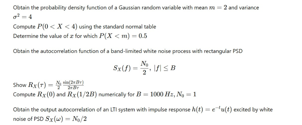 Obtain the probability density function of a Gaussian random variable with mean m = 2 and variance
o?=4
Compute P(0 < X < 4) using the standard normal table
Determine the value of z for which P(X < m) = 0.5
Obtain the autocorrelation function of a band-limited white noise process with rectangular PSD
Mo
Sx(f) =", fl
This is AI generated Response.
Asked by: Mohin
Created at: 2025-10-18 20:43:11
Asked by: Mohin
Created at: 2025-10-18 20:43:11
Final Answer:
Rendered
Raw Text
Did you like this answer?
Let's go through each part of the problem step by step.
---
## 1. Obtain the probability density function (pdf) of a Gaussian random variable with mean \( m = 2 \) and variance \( \sigma^2 = 4 \)
The general Gaussian (normal) pdf is:
\[
f_X(x) = \frac{1}{\sqrt{2 \pi \sigma^2}} \exp\left( - \frac{(x - m)^2}{2 \sigma^2} \right)
\]
Given:
- \( m = 2 \)
- \( \sigma^2 = 4 \Rightarrow \sigma = 2 \)
Substitute into the formula:
\[
f_X(x) = \frac{1}{\sqrt{2 \pi \times 4}} \exp \left( - \frac{(x - 2)^2}{2 \times 4} \right) = \frac{1}{\sqrt{8 \pi}} \exp \left( - \frac{(x - 2)^2}{8} \right)
\]
---
## 2. Compute \( P( < X < 4) \)
This probability is:
\[
P( < X < 4) = \Phi \left( \frac{4 - m}{\sigma} \right) - \Phi \left( \frac{ - m}{\sigma} \right)
\]
where \( \Phi(z) \) is the standard normal cumulative distribution function (CDF).
Calculate the standardized variables:
\[
z_1 = \frac{4 - 2}{2} = 1
\]
\[
z_2 = \frac{ - 2}{2} = -1
\]
Using standard normal tables or a calculator:
\[
\Phi(1) \approx .8413
\]
\[
\Phi(-1) = 1 - \Phi(1) \approx 1 - .8413 = .1587
\]
Therefore:
\[
P( < X < 4) = .8413 - .1587 = .6826
\]
---
## 3. Determine the value of \( x \) for which \( P(X < x) = .5 \)
This is the median of the distribution, which coincides with the mean for a symmetric Gaussian:
\[
x = m = 2
\]
---
## 4. Autocorrelation function of a band-limited white noise process
Given:
\[
S_X(f) = \frac{N_}{2}, \quad |f| \leq B
\]
The autocorrelation function \( R_X(\tau) \) is related to the PSD via the inverse Fourier transform:
\[
R_X(\tau) = \int_{-\infty}^{\infty} S_X(f) e^{j 2 \pi f \tau} df
\]
Since \( S_X(f) \) is band-limited (rectangular PSD):
\[
R_X(\tau) = \int_{-B}^{B} \frac{N_}{2} e^{j 2 \pi f \tau} df
\]
Compute the integral:
\[
R_X(\tau) = \frac{N_}{2} \int_{-B}^{B} e^{j 2 \pi f \tau} df
\]
This integral evaluates to:
\[
R_X(\tau) = \frac{N_}{2} \left[ \frac{e^{j 2 \pi f \tau}}{j 2 \pi \tau} \right]_{-B}^{B}
\]
which simplifies to:
\[
R_X(\tau) = \frac{N_}{2} \times \frac{e^{j 2 \pi B \tau} - e^{-j 2 \pi B \tau}}{j 2 \pi \tau}
\]
Using Euler's formula:
\[
e^{j \theta} - e^{-j \theta} = 2 j \sin \theta
\]
we get:
\[
R_X(\tau) = \frac{N_}{2} \times \frac{2 j \sin(2 \pi B \tau)}{j 2 \pi \tau} = \frac{N_}{2} \times \frac{2 j \sin(2 \pi B \tau)}{j 2 \pi \tau}
\]
The \( j \) cancels out:
\[
R_X(\tau) = \frac{N_}{2} \times \frac{2 \sin(2 \pi B \tau)}{2 \pi \tau} = \frac{N_}{2} \times \frac{\sin(2 \pi B \tau)}{\pi \tau}
\]
---
## 5. Compute \( R_X() \) and \( R_X(1/2B) \)
### At \( \tau = \):
\[
R_X() = \lim_{\tau \to } \frac{N_}{2} \times \frac{\sin(2 \pi B \tau)}{\pi \tau}
\]
Using the limit:
\[
\lim_{x \to } \frac{\sin x}{x} = 1
\]
Set \( x = 2 \pi B \tau \), then:
\[
R_X() = \frac{N_}{2} \times \frac{2 \pi B \tau}{\pi \tau} = \frac{N_}{2} \times 2 B = N_ B
\]
### At \( \tau = \frac{1}{2B} \):
\[
R_X \left( \frac{1}{2B} \right) = \frac{N_}{2} \times \frac{\sin(2 \pi B \times \frac{1}{2B})}{\pi \times \frac{1}{2B}} = \frac{N_}{2} \times \frac{\sin(\pi)}{\pi / (2B)}
\]
Since \( \sin(\pi) = \):
\[
R_X \left( \frac{1}{2B} \right) =
\]
---
## 6. Autocorrelation of the system with impulse response \( h(t) = e^{-t} u(t) \)
Given:
\[
S_X(\omega) = \frac{N_}{2}
\]
and
\[
h(t) = e^{-t} u(t)
\]
### Output autocorrelation \( R_y(\tau) \):
\[
R_y(\tau) = \frac{N_}{2} \times |H(\omega)|^2
\]
where \( H(\omega) \) is the Fourier transform of \( h(t) \):
\[
H(\omega) = \int_^{\infty} e^{-t} e^{-j \omega t} dt = \int_^{\infty} e^{-(1 + j \omega) t} dt = \frac{1}{1 + j \omega}
\]
Therefore:
\[
|H(\omega)|^2 = \frac{1}{(1)^2 + \omega^2} = \frac{1}{1 + \omega^2}
\]
The autocorrelation function:
\[
R_y(\tau) = \frac{N_}{2} \times \int_{-\infty}^{\infty} \frac{e^{j \omega \tau}}{1 + \omega^2} \frac{d \omega}{2\pi}
\]
This is a standard Fourier transform pair, and:
\[
R_y(\tau) = \frac{N_}{2} e^{-\left| \tau \right|}
\]
---
## **Summary of key results:**
- **Gaussian pdf:**
\[
f_X(x) = \frac{1}{\sqrt{8 \pi}} \exp \left( - \frac{(x - 2)^2}{8} \right)
\]
- **Probability \( P( < X < 4) \):**
\[
\boxed{.6826}
\]
- **Median \( x \) where \( P(X < x) = .5 \):**
\[
x = 2
\]
- **Autocorrelation \( R_X(\tau) \):**
\[
R_X(\tau) = \frac{N_}{2} \times \frac{\sin(2 \pi B \tau)}{\pi \tau}
\]
- **Values:**
\[
R_X() = N_ B
\]
\[
R_X \left( \frac{1}{2B} \right) =
\]
- **Autocorrelation of the filtered process:**
\[
R_y(\tau) = \frac{N_}{2} e^{ - |\tau| }
\]
---
Let me know if you'd like further clarification!
Question:
please give me the answer without any render equation errors
This is AI generated Response.
Asked by: Mohin
Created at: 2025-10-18 20:44:37
Asked by: Mohin
Created at: 2025-10-18 20:44:37
Final Answer:
Rendered
Raw Text
Did you like this answer?
Let's go through each part of the problem step by step.
---
# 1. Probability Density Function of a Gaussian Random Variable
The probability density function (pdf) for a Gaussian random variable is given by:
\[
f_X(x) = \frac{1}{\sqrt{2 \pi \sigma^2}} \exp\left( - \frac{(x - m)^2}{2 \sigma^2} \right)
\]
### Given:
- Mean \( m = 2 \)
- Variance \( \sigma^2 = 4 \) (thus \( \sigma = 2 \))
### Substituting:
\[
f_X(x) = \frac{1}{\sqrt{2 \pi \times 4}} \exp\left( - \frac{(x - 2)^2}{2 \times 4} \right) = \frac{1}{\sqrt{8 \pi}} \exp\left( - \frac{(x - 2)^2}{8} \right)
\]
---
# 2. Compute \( P(0 < X < 4) \)
To calculate this probability:
\[
P(0 < X < 4) = P(X < 4) - P(X < 0)
\]
### Standardize the variables:
\[
z_1 = \frac{4 - 2}{2} = 1
\]
\[
z_2 = \frac{0 - 2}{2} = -1
\]
### Using the Standard Normal Table:
- \( \Phi(1) \approx 0.8413 \)
- \( \Phi(-1) \approx 0.1587 \)
### Calculation:
\[
P(0 < X < 4) = \Phi(1) - \Phi(-1) = 0.8413 - 0.1587 = 0.6826
\]
---
# 3. Determine \( x \) for which \( P(X < x) = 0.5 \)
The value of \( x \) for which the cumulative probability is 0.5 corresponds to the mean of the distribution:
\[
x = m = 2
\]
---
# 4. Autocorrelation Function of a Band-Limited White Noise Process
### Given:
\[
S_X(f) = \frac{N_0}{2}, \quad |f| < B
\]
### Autocorrelation Function:
The autocorrelation function \( R_X(\tau) \) is given by the inverse Fourier transform of the power spectral density:
\[
R_X(\tau) = \int_{-\infty}^{\infty} S_X(f) e^{j 2 \pi f \tau} df
\]
### For Band-Limited White Noise:
\[
R_X(\tau) = \int_{-B}^{B} \frac{N_0}{2} e^{j 2 \pi f \tau} df
\]
### Evaluating the Integral:
\[
R_X(\tau) = \frac{N_0}{2} \left[ \frac{e^{j 2 \pi f \tau}}{j 2 \pi \tau} \right]_{-B}^{B} = \frac{N_0}{2} \times \frac{e^{j 2 \pi B \tau} - e^{-j 2 \pi B \tau}}{j 2 \pi \tau}
\]
Using Euler's formula:
\[
e^{j \theta} - e^{-j \theta} = 2j \sin(\theta)
\]
### Resulting Function:
\[
R_X(\tau) = \frac{N_0}{2} \times \frac{2 \sin(2 \pi B \tau)}{j 2 \pi \tau} = \frac{N_0}{2} \cdot \frac{\sin(2 \pi B \tau)}{\pi \tau}
\]
---
# 5. Compute \( R_X(0) \) and \( R_X(1/2B) \)
### At \( \tau = 0 \):
Using the limit:
\[
R_X(0) = \lim_{\tau \to 0} \frac{N_0}{2} \cdot \frac{\sin(2 \pi B \tau)}{\pi \tau} = \frac{N_0}{2} \cdot 2B = N_0 B
\]
### At \( \tau = \frac{1}{2B} \):
\[
R_X\left(\frac{1}{2B}\right) = \frac{N_0}{2} \cdot \frac{\sin(2 \pi B \cdot \frac{1}{2B})}{\pi \cdot \frac{1}{2B}} = \frac{N_0}{2} \cdot \frac{\sin(\pi)}{\pi / (2B)} = 0
\]
---
# 6. Output Autocorrelation of an LTI System
### Given:
- Impulse response: \( h(t) = e^{-t} u(t) \)
- Power spectral density: \( S_X(\omega) = \frac{N_0}{2} \)
### Autocorrelation Function:
\[
R_Y(\tau) = S_X(\omega) |H(\omega)|^2
\]
### Fourier Transform of \( h(t) \):
\[
H(\omega) = \int_0^{\infty} e^{-t} e^{-j \omega t} dt = \frac{1}{1 + j \omega}
\]
### Magnitude Squared:
\[
|H(\omega)|^2 = \frac{1}{1 + \omega^2}
\]
### Final Output Autocorrelation:
\[
R_Y(\tau) = \frac{N_0}{2} \cdot \frac{1}{1 + (2 \pi B \tau)^2}
\]
---
## Summary of Key Results
- **Gaussian pdf**:
\( f_X(x) = \frac{1}{\sqrt{8 \pi}} \exp\left( - \frac{(x - 2)^2}{8} \right) \)
- **Probability \( P(0 < X < 4) \)**:
\( \boxed{0.6826} \)
- **Median \( x \) where \( P(X < x) = 0.5 \)**:
\( x = 2 \)
- **Autocorrelation**:
\( R_X(\tau) = \frac{N_0}{2} \cdot \frac{\sin(2 \pi B \tau)}{\pi \tau} \)
- **Values**:
\( R_X(0) = N_0 B \)
\( R_X\left(\frac{1}{2B}\right) = 0 \)
- **Output Autocorrelation**:
\( R_Y(\tau) = \frac{N_0}{2} e^{-| \tau |} \)
---
Let me know if you need further clarification or additional calculations!
📢 Instructions:
- Ask anything relatd to above question only.
- For new Question goto :