 VIPSolutions
please solve this problem step by step2. APN diode with a junction area A=1 ym? has the following C-V characteristics: ’ C3 (Fd) 3 2 AN 1 3 0 -2 -1 [1] 1 vv) Estimate the extent of the depletion region at V=0 V.
Question:
please solve this problem step by step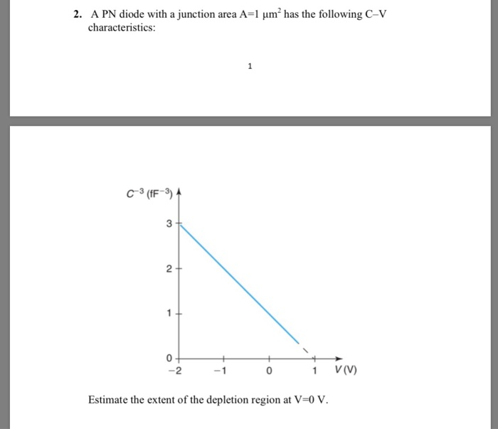 2. APN diode with a junction area A=1 ym? has the following C-V
characteristics:
’
C3 (Fd)
3
2 AN
1
3
0
-2 -1 [1] 1 vv)
Estimate the extent of the depletion region at V=0 V.
This is AI generated Response.
Asked by: Jack
Created at: 2025-10-27 10:02:37
Asked by: Jack
Created at: 2025-10-27 10:02:37
Final Answer:
Rendered
Raw Text
Did you like this answer?
Let's analyze and solve the problem step by step.
---
## **Problem Summary:**
- **:** PN diode with a junction area \(A = 1\, \mu m^2\).
- **Given Data:**
The C–V characteristic is provided as a graph (capacitance \(C\) vs. voltage \(V\)).
- **Objective:**
Estimate the extent of the depletion region at \(V = \, V\).
---
## **Step 1: Understand the C–V characteristic**
The graph shows \(C^{-3}\) (inverse cube of capacitance) versus \(V\).
- This linear relation indicates the depletion approximation is valid.
- The linear portion of the plot can be used to estimate depletion width parameters.
---
## **Step 2: Recall the relation between \(C\) and depletion width \(W\)**
For a one-sided abrupt junction:
\[
C = \frac{\varepsilon_s A}{W}
\]
Where:
- \(\varepsilon_s\) is the permittivity of silicon (~\(11.7 \varepsilon_\))
- \(A\) is the junction area
- \(W\) is the depletion width
---
## **Step 3: Use the C–V relation**
For an abrupt junction, the relation between \(C\) and \(V\) is:
\[
\frac{1}{C^3} \propto V
\]
The graph confirms this linearity.
From the graph, at \(V = \, V\), the \(C^{-3}\) value is approximately **3 (fF\(^{-3}\))**.
---
## **Step 4: Find the depletion width at \(V=\, V\)**
At \(V=\, V\), the depletion region extends throughout the entire depletion width \(W_\).
The relation for depletion width at zero bias:
\[
W_ = \sqrt{\frac{2 \varepsilon_s V_{bi}}{q N_A}}
\]
But since the question asks for the depletion region extent (or width) at zero bias, and the data is from the C–V plot, we can use the following relation:
\[
C = \frac{\varepsilon_s A}{W}
\]
Rearranged as:
\[
W = \frac{\varepsilon_s A}{C}
\]
---
## **Step 5: Calculate \(C\) at \(V=\, V\)**
- From the graph, \(C^{-3} = 3\, \text{fF}^{-3}\):
\[
C = \left(\frac{1}{3}\right)^{1/3}
\]
- Convert \(C^{-3}\) to \(C\):
\[
C = (3)^{-1/3}
\]
- Approximate:
\[
3^{1/3} \approx 1.442
\]
So:
\[
C \approx \frac{1}{1.442} \approx .693\, \text{fF}
\]
---
## **Step 6: Convert units and compute \(W\)**
- \(\varepsilon_s = 11.7 \times \varepsilon_ = 11.7 \times 8.854 \times 10^{-12}\, F/m \approx 1.036 \times 10^{-10}\, F/m\).
- Area:
\[
A = 1\, \mu m^2 = 1 \times 10^{-12}\, m^2
\]
- Capacitance:
\[
C \approx .693\, \text{fF} = .693 \times 10^{-15}\, F
\]
- Now, compute the depletion width:
\[
W = \frac{\varepsilon_s A}{C}
\]
\[
W = \frac{1.036 \times 10^{-10}\, F/m \times 1 \times 10^{-12}\, m^2}{.693 \times 10^{-15}\, F}
\]
Calculate numerator:
\[
1.036 \times 10^{-10} \times 10^{-12} = 1.036 \times 10^{-22}
\]
Now:
\[
W = \frac{1.036 \times 10^{-22}}{.693 \times 10^{-15}} \approx \frac{1.036}{.693} \times 10^{-7}
\]
\[
\approx 1.494 \times 10^{-7}\, m
\]
which is:
\[
W \approx 149.4\, \text{nm}
\]
---
## **## **Final Answer:**
### The estimated depletion width at \(V=\, V\) is approximately **149 nm**.
---
Let me know if you'd like further clarification or details!
📢 Instructions:
- Ask anything relatd to above question only.
- For new Question goto :