Give step-by-step solution with explanation and final answer:Question 4
4.39. Consider the system of Figure P4.39 consisting of two pendulums coupled by a spring. Determine the
natural frequency and mode shapes. Plot the mode shapes as well as the solution to an initial condition
consisting of the first mode shape for k= 20 N/m, I= 0.5 m, and m= mz =10 kg, a= 0.1 m along the
pendulum.
I kN Ya
1
VA I
i i -
i I Figure P439 Two pendulums of the
101 16, same length connected by a spring used
! om ! my .
2 to model a machine part.
a) Usethe Equation of Motion
b) Uselagrange’s Equation
Question:
Give step-by-step solution with explanation and final answer:Question 4
4.39. Consider the system of Figure P4.39 consisting of two pendulums coupled by a spring. Determine the
natural frequency and mode shapes. Plot the mode shapes as well as the solution to an initial condition
consisting of the first mode shape for k= 20 N/m, I= 0.5 m, and m= mz =10 kg, a= 0.1 m along the
pendulum.
I kN Ya
1
VA I
i i -
i I Figure P439 Two pendulums of the
101 16, same length connected by a spring used
! om ! my .
2 to model a machine part.
a) Usethe Equation of Motion
b) Uselagrange’s Equation
This is AI generated Response.
Asked by: gvr
Created at: 2025-06-25 17:56:52
Final Answer:
RenderedRaw Text
Did you like this answer?
Let's solve the problem **step by step** for both the **Equation of Motion** method and **Lagrange's Equation** method for the coupled pendulum system.
---
## **Step 1: System Description**
- **Two pendulums** of equal mass \( m \), length \( l \), angular displacement \( \theta_1 \) and \( \theta_2 \).
- Coupled by a spring of stiffness \( k \) attached a distance \( a \) from the pivot.
- Given: \( k = 20\,\text{N/m} \), \( l = 0.5\,\text{m} \), \( m = 10\,\text{kg} \), \( a = 0.1\,\text{m} \).
---
## **a) Equation of Motion Approach**
### **1. Write Equations for Each Pendulum**
For small angles (\( \sin\theta \approx \theta \)):
#### **Restoring torque due to gravity:**
\[
\tau_g = -mg l \theta
\]
#### **Restoring torque due to spring:**
The horizontal displacement at distance \( a \) from the pivot is \( a\theta \).
- Spring extension: \( x_\text{spring} = a(\theta_1 - \theta_2) \)
- Force on mass: \( F = -k x_\text{spring} \)
- Torque = \( F \times a = -k a^2 (\theta_1 - \theta_2) \)
#### **Moment of inertia of each pendulum:**
\[
I = m l^2
\]
#### **Equation for \(\theta_1\):**
\[
I \ddot{\theta}_1 = -mg l \theta_1 - k a^2 (\theta_1 - \theta_2)
\]
\[
m l^2 \ddot{\theta}_1 + mg l \theta_1 + k a^2 (\theta_1 - \theta_2) = 0
\]
#### **Similarly for \(\theta_2\):**
\[
m l^2 \ddot{\theta}_2 + mg l \theta_2 + k a^2 (\theta_2 - \theta_1) = 0
\]
---
### **2. Express in Matrix Form:**
\[
m l^2 \begin{bmatrix} \ddot{\theta}_1 \\ \ddot{\theta}_2 \end{bmatrix} +
\begin{bmatrix}
mg l + k a^2 & -k a^2 \\
-k a^2 & mg l + k a^2
\end{bmatrix}
\begin{bmatrix} \theta_1 \\ \theta_2 \end{bmatrix}
= 0
\]
---
### **3. Find Natural Frequencies and Mode Shapes**
Assume solution: \( \theta_i = A_i e^{i \omega t} \)
\[
\left[ -m l^2 \omega^2 \mathbf{I} +
\begin{bmatrix}
mg l + k a^2 & -k a^2 \\
-k a^2 & mg l + k a^2
\end{bmatrix}
\right]
\begin{bmatrix} A_1 \\ A_2 \end{bmatrix} = 0
\]
Set determinant to zero for non-trivial solutions:
\[
\left|
\begin{matrix}
mg l + k a^2 - m l^2 \omega^2 & -k a^2 \\
-k a^2 & mg l + k a^2 - m l^2 \omega^2
\end{matrix}
\right| = 0
\]
\[
\left(mg l + k a^2 - m l^2 \omega^2\right)^2 - (k a^2)^2 = 0
\]
\[
mg l + k a^2 - m l^2 \omega^2 = \pm k a^2
\]
\[
mg l + k a^2 - m l^2 \omega^2 = k a^2 \implies mg l - m l^2 \omega^2 = 0 \implies \omega_1^2 = \frac{g}{l}
\]
\[
mg l + k a^2 - m l^2 \omega^2 = -k a^2 \implies mg l + 2k a^2 - m l^2 \omega^2 = 0 \implies \omega_2^2 = \frac{g}{l} + \frac{2k a^2}{ml^2}
\]
---
### **4. Mode Shapes**
For \( \omega_1^2 = \frac{g}{l} \):
\[
\left[ mg l + k a^2 - m l^2 \omega_1^2 \right] A_1 - k a^2 A_2 = 0
\]
\[
k a^2 (A_1 - A_2) = 0 \implies A_1 = A_2
\]
**Mode 1:** \([1, 1]^T\) (in-phase)
For \( \omega_2^2 = \frac{g}{l} + \frac{2k a^2}{ml^2} \):
\[
\left[ mg l + k a^2 - m l^2 \omega_2^2 \right] A_1 - k a^2 A_2 = 0
\]
\[
- k a^2 (A_1 + A_2) = 0 \implies A_1 = -A_2
\]
**Mode 2:** \([1, -1]^T\) (out-of-phase)
---
### **5. Numerical Values**
- \( g = 9.81\,\text{m/s}^2 \)
- \( k = 20\,\text{N/m} \)
- \( a = 0.1\,\text{m} \)
- \( m = 10\,\text{kg} \)
- \( l = 0.5\,\text{m} \)
\[
\omega_1^2 = \frac{9.81}{0.5} = 19.62 \implies \omega_1 = 4.432\,\text{rad/s}
\]
\[
\omega_2^2 = \frac{9.81}{0.5} + \frac{2 \times 20 \times (0.1)^2}{10 \times (0.5)^2} = 19.62 + \frac{0.4}{2.5} = 19.62 + 0.16 = 19.78
\]
\[
\omega_2 = 4.449\,\text{rad/s}
\]
---
### **6. Plotting Mode Shapes**
- **First Mode:** Both pendulums swing together
- **Second Mode:** Pendulums swing opposite to each other
---
## **b) Using Lagrange’s Equation**
### **1. Kinetic Energy**
Each mass:
\[
T = \frac{1}{2} m (l^2 \dot{\theta}_1^2 + l^2 \dot{\theta}_2^2) = \frac{1}{2} m l^2 (\dot{\theta}_1^2 + \dot{\theta}_2^2)
\]
### **2. Potential Energy**
- **Gravity:** \( V_g = m g l (1 - \cos \theta) \approx \frac{1}{2} m g l \theta^2 \)
- **Spring:** \( V_s = \frac{1}{2} k (a(\theta_1 - \theta_2))^2 = \frac{1}{2} k a^2 (\theta_1 - \theta_2)^2 \)
\[
V = \frac{1}{2} m g l \theta_1^2 + \frac{1}{2} m g l \theta_2^2 + \frac{1}{2} k a^2 (\theta_1 - \theta_2)^2
\]
---
### **3. Lagrangian**
\[
L = T - V
\]
Write Lagrange’s equations for \( \theta_1 \), \( \theta_2 \):
\[
\frac{d}{dt} \left( \frac{\partial L}{\partial \dot{\theta}_i} \right) - \frac{\partial L}{\partial \theta_i} = 0
\]
Yields the same equations of motion as above.
---
## **Summary Table**
| Mode | Natural Frequency (\(\omega\)) | Mode Shape |
|------|-------------------------------|--------------------|
| 1 | \(4.432\,\text{rad/s}\) | \(\begin{bmatrix}1 \\ 1\end{bmatrix}\) |
| 2 | \(4.449\,\text{rad/s}\) | \(\begin{bmatrix}1 \\ -1\end{bmatrix}\) |
---
## **Plotting (Python Example)**
```python
import numpy as np
import matplotlib.pyplot as plt
# Mode shapes
mode1 = np.array([1, 1])
mode2 = np.array([1, -1])
plt.figure()
plt.plot([0, 1], mode1, label='Mode 1 (In-phase)')
plt.plot([0, 1], mode2, label='Mode 2 (Out-of-phase)')
plt.xticks([0, 1], ['Pendulum 1', 'Pendulum 2'])
plt.ylabel('Amplitude')
plt.legend()
plt.title('Mode Shapes of Coupled Pendulums')
plt.grid(True)
plt.show()
```
---
## **Final Answer**
- **Natural Frequencies:** \( \omega_1 = 4.432\,\text{rad/s} \), \( \omega_2 = 4.449\,\text{rad/s} \)
- **Mode Shapes:** Mode 1: [1, 1], Mode 2: [1, -1]
- **Equations derived using both Newton's equations and Lagrange's equations match.**
If you require the **solution to a specific initial condition** or the **full time response**, let me know!
Question:
i need detailed calculations along with the final Answer
This is AI generated Response.
Asked by: gvr
Created at: 2025-06-25 17:59:59
Final Answer:
RenderedRaw Text
Did you like this answer?
Certainly! Let's proceed with a detailed, step-by-step solution including all calculations, leading to the final answers.
---
### **Given Data:**
| Parameter | Value |
|---|---|
| Spring constant, \(k\) | 20 N/m |
| Length of pendulum, \(l\) | 0.5 m |
| Mass of each pendulum, \(m\) | 10 kg |
| Distance from pivot to spring attachment point, \(a\) | 0.1 m |
| Acceleration due to gravity, \(g\) | 9.81 m/s² |
---
## **Part A: Equation of Motion Approach**
### **Step 1: Model assumptions**
- Small-angle approximation: \(\sin \theta \approx \theta\)
- Each pendulum's angular displacement: \(\theta_1(t)\) and \(\theta_2(t)\)
### **Step 2: Derive equations of motion**
**For each pendulum, the torque equation:**
\[
I \ddot{\theta}_i = \text{Restoring torque due to gravity} + \text{Spring torque}
\]
where the moment of inertia:
\[
I = m l^2
\]
---
### **Step 3: Write the torque contributions**
- **Gravity torque:**
\[
\tau_g = - m g l \theta_i
\]
- **Spring torque:**
The horizontal displacement at the spring attachment point:
\[
x_i = a \theta_i
\]
The extension/compression of the spring:
\[
x_{\text{spring}} = x_1 - x_2 = a (\theta_1 - \theta_2)
\]
Spring force:
\[
F_s = -k x_{\text{spring}} = -k a (\theta_1 - \theta_2)
\]
Torque about the pivot for each pendulum:
\[
\tau_s = F_s \times a = -k a^2 (\theta_1 - \theta_2)
\]
---
### **Step 4: Write the equations**
For pendulum 1:
\[
m l^2 \ddot{\theta}_1 + m g l \theta_1 + k a^2 (\theta_1 - \theta_2) = 0
\]
For pendulum 2:
\[
m l^2 \ddot{\theta}_2 + m g l \theta_2 + k a^2 (\theta_2 - \theta_1) = 0
\]
---
### **Step 5: Matrix form**
Define:
\[
\mathbf{\Theta} = \begin{bmatrix} \theta_1 \\ \theta_2 \end{bmatrix}
\]
The equations:
\[
m l^2 \ddot{\mathbf{\Theta}} + \mathbf{K} \mathbf{\Theta} = 0
\]
where the stiffness matrix:
\[
\mathbf{K} = \begin{bmatrix}
m g l + k a^2 & -k a^2 \\
-k a^2 & m g l + k a^2
\end{bmatrix}
\]
---
### **Step 6: Numerical substitution**
Calculate constants:
\[
m g l = 10 \times 9.81 \times 0.5 = 49.05\, \text{Nm}
\]
\[
k a^2 = 20 \times (0.1)^2 = 20 \times 0.01 = 0.2\, \text{Nm}
\]
So,
\[
\mathbf{K} = \begin{bmatrix}
49.05 + 0.2 & -0.2 \\
-0.2 & 49.05 + 0.2
\end{bmatrix} = \begin{bmatrix}
49.25 & -0.2 \\
-0.2 & 49.25
\end{bmatrix}
\]
Moment of inertia:
\[
I = m l^2 = 10 \times (0.5)^2 = 10 \times 0.25 = 2.5\, \text{kg·m}^2
\]
---
### **Step 7: Eigenvalue problem**
Assuming solution:
\[
\mathbf{\Theta}(t) = \mathbf{A} e^{i \omega t}
\]
Substituting into the equations:
\[
- \omega^2 I \mathbf{A} + \mathbf{K} \mathbf{A} = 0
\]
\[
(\mathbf{K} - \omega^2 I \mathbf{I}) \mathbf{A} = 0
\]
Non-trivial solutions require:
\[
\det (\mathbf{K} - \omega^2 I \mathbf{I}) = 0
\]
which simplifies to:
\[
\det \left( \begin{bmatrix}
49.25 - 2.5 \omega^2 & -0.2 \\
-0.2 & 49.25 - 2.5 \omega^2
\end{bmatrix} \right) = 0
\]
---
### **Step 8: Determinant calculation**
\[
(49.25 - 2.5 \omega^2)^2 - (-0.2)^2 = 0
\]
\[
(49.25 - 2.5 \omega^2)^2 - 0.04 = 0
\]
\[
(49.25 - 2.5 \omega^2)^2 = 0.04
\]
Take square root:
\[
49.25 - 2.5 \omega^2 = \pm 0.2
\]
---
### **Step 9: Solve for \(\omega^2\)**
**Case 1:**
\[
49.25 - 2.5 \omega^2 = 0.2
\]
\[
2.5 \omega^2 = 49.25 - 0.2 = 49.05
\]
\[
\omega^2 = \frac{49.05}{2.5} = 19.62
\]
\[
\boxed{\omega_1 = \sqrt{19.62} \approx 4.43\, \text{rad/sec}}
\]
**Case 2:**
\[
49.25 - 2.5 \omega^2 = -0.2
\]
\[
2.5 \omega^2 = 49.25 + 0.2 = 49.45
\]
\[
\omega^2 = \frac{49.45}{2.5} = 19.78
\]
\[
\boxed{\omega_2 = \sqrt{19.78} \approx 4.45\, \text{rad/sec}}
\]
---
## **Part B: Mode Shapes**
From the eigenvalue equations:
\[
(49.25 - 2.5 \omega^2) A_1 - 0.2 A_2 = 0
\]
For \(\omega_1^2 = 19.62\):
\[
49.25 - 2.5 \times 19.62 = 49.25 - 49.05 = 0.2
\]
Equation:
\[
0.2 A_1 - 0.2 A_2 = 0 \Rightarrow A_1 = A_2
\]
**Mode shape 1:** \(\boxed{[1, 1]} \) (both pendulums oscillate in phase)
For \(\omega_2^2 = 19.78\):
\[
49.25 - 2.5 \times 19.78 = 49.25 - 49.45 = -0.2
\]
Equation:
\[
-0.2 A_1 - 0.2 A_2 = 0 \Rightarrow A_1 = -A_2
\]
**Mode shape 2:** \(\boxed{[1, -1]} \) (oscillations out of phase)
---
## **Final Results:**
| **Mode** | **Frequency \(\omega\) (rad/sec)** | **Mode Shape** |
|------------|----------------------------------|----------------|
| **1** | \( \boxed{4.43} \) | \([1, 1]\) (in-phase) |
| **2** | \( \boxed{4.45} \) | \([1, -1]\) (out-of-phase) |
---
## **Plotting Mode Shapes:**
The mode shapes indicate how the pendulums oscillate relative to each other:
- **Mode 1:** Both swing together with the same amplitude.
- **Mode 2:** Pendulums swing opposite to each other with equal amplitude.
---
## **Summary:**
- The **natural frequencies** are approximately **4.43 rad/sec** and **4.45 rad/sec**.
- The **mode shapes** are **in-phase** \([1, 1]\) and **out-of-phase** \([1, -1]\).
---
**Note:** To find the **time response** for specific initial conditions, you would decompose the initial displacements into these modes and superimpose their solutions, but that would require additional initial data.
---
If further clarifications or calculations are needed, feel free to ask!
Question:
please genarte the answer with detailed calculations and derivations explanations along with the final Answer no need any tables
This is AI generated Response.
Asked by: gvr
Created at: 2025-06-25 18:08:27
Final Answer:
RenderedRaw Text
Did you like this answer?
Certainly! Here is a comprehensive, step-by-step solution with detailed calculations, derivations, and explanations for the problem involving two coupled pendulums connected by a spring.
---
### **System Description**
We have two identical pendulums of mass \( m = 10\, \mathrm{kg} \), length \( l = 0.5\, \mathrm{m} \), connected by a spring with stiffness \( k = 20\, \mathrm{N/m} \). The spring is attached at a point \( a = 0.1\, \mathrm{m} \) from each pivot. The goal is to find the natural frequencies and mode shapes of the system.
---
### **Part A: Derivation of Equations of Motion**
#### **1. Assumptions and Coordinates**
Assuming small oscillations, the angular displacements \( \theta_1(t) \) and \( \theta_2(t) \) of the two pendulums are small, enabling linearization. The angular displacements are measured from the vertical.
Each pendulum's kinetic energy (due to rotation about the pivot):
\[
T = \frac{1}{2} I \dot{\theta}_i^2,
\]
where the moment of inertia \( I = m l^2 = 10 \times (0.5)^2 = 2.5\, \mathrm{kg\,m^2} \).
Total kinetic energy:
\[
T = \frac{1}{2} I (\dot{\theta}_1^2 + \dot{\theta}_2^2).
\]
#### **2. Potential Energy Components**
- **Gravity:** For small angles, the potential energy relative to the lowest position:
\[
V_g = m g l (1 - \cos \theta) \approx \frac{1}{2} m g l \theta^2,
\]
so the total gravitational potential energy:
\[
V_{g} = \frac{1}{2} m g l (\theta_1^2 + \theta_2^2).
\]
- **Spring:** The spring connects points at a distance \( a \) from each pivot, with horizontal displacement \( x_i = a \theta_i \).
The extension or compression of the spring is:
\[
x_1 - x_2 = a (\theta_1 - \theta_2).
\]
The spring's potential energy:
\[
V_s = \frac{1}{2} k (x_1 - x_2)^2 = \frac{1}{2} k a^2 (\theta_1 - \theta_2)^2.
\]
Total potential energy:
\[
V = V_g + V_s = \frac{1}{2} m g l (\theta_1^2 + \theta_2^2) + \frac{1}{2} k a^2 (\theta_1 - \theta_2)^2.
\]
---
### **Part B: Deriving Equations of Motion**
The Lagrangian:
\[
L = T - V = \frac{1}{2} I (\dot{\theta}_1^2 + \dot{\theta}_2^2) - \left[ \frac{1}{2} m g l (\theta_1^2 + \theta_2^2) + \frac{1}{2} k a^2 (\theta_1 - \theta_2)^2 \right].
\]
Applying Lagrange's equations:
\[
\frac{d}{dt} \left( \frac{\partial L}{\partial \dot{\theta}_i} \right) - \frac{\partial L}{\partial \theta_i} = 0,
\]
for \( i = 1, 2 \).
Calculate derivatives:
\[
\frac{\partial L}{\partial \dot{\theta}_i} = I \dot{\theta}_i,
\]
\[
\frac{d}{dt} \left( I \dot{\theta}_i \right) = I \ddot{\theta}_i,
\]
\[
\frac{\partial L}{\partial \theta_1} = - m g l \theta_1 - k a^2 (\theta_1 - \theta_2),
\]
\[
\frac{\partial L}{\partial \theta_2} = - m g l \theta_2 - k a^2 (\theta_2 - \theta_1).
\]
Thus, equations of motion:
\[
I \ddot{\theta}_1 + m g l \theta_1 + k a^2 (\theta_1 - \theta_2) = 0,
\]
\[
I \ddot{\theta}_2 + m g l \theta_2 + k a^2 (\theta_2 - \theta_1) = 0.
\]
---
### **Part C: Expressing in Matrix Form**
Define the displacement vector:
\[
\boldsymbol{\Theta} = \begin{bmatrix} \theta_1 \\ \theta_2 \end{bmatrix}.
\]
The equations become:
\[
I \ddot{\boldsymbol{\Theta}} + \mathbf{K} \boldsymbol{\Theta} = 0,
\]
where the stiffness matrix:
\[
\mathbf{K} = \begin{bmatrix}
m g l + k a^2 & -k a^2 \\
-k a^2 & m g l + k a^2
\end{bmatrix}.
\]
Substituting the known values:
\[
m g l = 10 \times 9.81 \times 0.5 = 49.05\, \mathrm{Nm},
\]
\[
k a^2 = 20 \times (0.1)^2 = 0.2\, \mathrm{Nm}.
\]
So,
\[
\mathbf{K} = \begin{bmatrix}
49.05 + 0.2 & -0.2 \\
-0.2 & 49.05 + 0.2
\end{bmatrix} = \begin{bmatrix}
49.25 & -0.2 \\
-0.2 & 49.25
\end{bmatrix}.
\]
---
### **Part D: Finding Natural Frequencies**
Assuming harmonic motion:
\[
\boldsymbol{\Theta}(t) = \mathbf{A} e^{i \omega t},
\]
which yields:
\[
- \omega^2 I \mathbf{A} + \mathbf{K} \mathbf{A} = 0,
\]
or equivalently:
\[
(\mathbf{K} - \omega^2 I \mathbf{I}) \mathbf{A} = 0.
\]
Non-trivial solutions exist when:
\[
\det (\mathbf{K} - \omega^2 I \mathbf{I}) = 0.
\]
Calculating:
\[
\det \begin{bmatrix}
49.25 - 2.5 \omega^2 & -0.2 \\
-0.2 & 49.25 - 2.5 \omega^2
\end{bmatrix} = 0.
\]
The determinant:
\[
(49.25 - 2.5 \omega^2)^2 - (-0.2)^2 = 0,
\]
\[
(49.25 - 2.5 \omega^2)^2 = 0.04,
\]
\[
49.25 - 2.5 \omega^2 = \pm 0.2.
\]
Now, solve for \( \omega^2 \):
**Case 1:**
\[
49.25 - 2.5 \omega^2 = 0.2,
\]
\[
2.5 \omega^2 = 49.25 - 0.2 = 49.05,
\]
\[
\omega^2 = \frac{49.05}{2.5} = 19.62,
\]
\[
\omega_{1} = \sqrt{19.62} \approx 4.43\, \mathrm{rad/sec}.
\]
**Case 2:**
\[
49.25 - 2.5 \omega^2 = -0.2,
\]
\[
2.5 \omega^2 = 49.25 + 0.2 = 49.45,
\]
\[
\omega^{2} = \frac{49.45}{2.5} = 19.78,
\]
\[
\omega_{2} = \sqrt{19.78} \approx 4.45\, \mathrm{rad/sec}.
\]
---
### **Part E: Mode Shapes**
To find mode shapes, substitute \( \omega^2 \) back into the eigenvalue equation:
\[
(49.25 - 2.5 \omega^2) A_1 - 0.2 A_2 = 0.
\]
For \( \omega_1^2 = 19.62 \):
\[
49.25 - 2.5 \times 19.62 = 49.25 - 49.05 = 0.2,
\]
\[
0.2 A_1 - 0.2 A_2 = 0,
\]
\[
A_1 = A_2.
\]
This indicates an **in-phase mode**: both pendulums swing together with the same amplitude.
For \( \omega_2^2 = 19.78 \):
\[
49.25 - 2.5 \times 19.78 = 49.25 - 49.45 = -0.2,
\]
\[
-0.2 A_1 - 0.2 A_2 = 0,
\]
\[
A_1 = -A_2,
\]
which indicates an **out-of-phase mode**: pendulums swing opposite to each other with equal amplitude.
---
### **Final Results**
The **natural frequencies** are approximately **4.43 rad/sec** for the in-phase mode, and **4.45 rad/sec** for the out-of-phase mode.
The **mode shapes** are:
- In-phase: both pendulums oscillate together, corresponding to eigenvector \([1, 1]\).
- Out-of-phase: pendulums oscillate opposite to each other, eigenvector \([1, -1]\).
---
### **Summary**
The two coupled pendulums have very close natural frequencies, with the in-phase mode at approximately 4.43 rad/sec and the out-of-phase mode at approximately 4.45 rad/sec. The mode shapes confirm that in the first mode, both pendulums swing in unison, while in the second, they swing in opposition.
This detailed derivation combines physical modeling, linearization, matrix eigenvalue analysis, and interpretation of mode shapes, providing a complete understanding of the system's vibrational characteristics.
---
If you need further analysis, such as the response to specific initial conditions or plots of the mode shapes, please let me know!
Question:
i need detailed explanation and calculations of each part along with the final Answer
This is AI generated Response.
Asked by: gvr
Created at: 2025-06-25 18:16:48
Final Answer:
RenderedRaw Text
Did you like this answer?
Certainly! Here is a detailed, step-by-step explanation with all calculations, derivations, and reasoning, culminating in the final answer for the coupled pendulum system.
---
### **System Overview**
We have two identical pendulums of mass \(m=10\, \mathrm{kg}\), length \(l=0.5\, \mathrm{m}\), connected via a spring of stiffness \(k=20\, \mathrm{N/m}\). The spring attaches at a point \(a=0.1\, \mathrm{m}\) from each pivot on both pendulums. Our goal is to find the system's natural frequencies and mode shapes.
---
### **Part 1: Deriving Equations of Motion**
**Assumptions:**
- Small oscillations, so \(\sin \theta \approx \theta\).
- The angular displacements are \(\theta_1(t)\) and \(\theta_2(t)\).
**Kinetic Energy:**
Each pendulum's kinetic energy:
\[
T_i = \frac{1}{2} I \dot{\theta}_i^2,
\]
where the moment of inertia for a point mass at the end of a massless rod:
\[
I = m l^2 = 10 \times (0.5)^2 = 2.5\, \mathrm{kg\,m^2}.
\]
Total kinetic energy:
\[
T = \frac{1}{2} I (\dot{\theta}_1^2 + \dot{\theta}_2^2).
\]
---
**Potential Energy:**
1. **Gravity:**
\[
V_g = m g l \left(1 - \cos \theta_i \right) \approx \frac{1}{2} m g l \theta_i^2,
\]
so total gravitational potential energy:
\[
V_{g} = \frac{1}{2} m g l (\theta_1^2 + \theta_2^2).
\]
2. **Spring:**
The spring exerts a restoring force proportional to the difference in horizontal displacements at the attachment points:
\[
x_i = a \theta_i,
\]
so the extension or compression of the spring:
\[
x_1 - x_2 = a (\theta_1 - \theta_2).
\]
Spring potential energy:
\[
V_s = \frac{1}{2} k (x_1 - x_2)^2 = \frac{1}{2} k a^2 (\theta_1 - \theta_2)^2.
\]
---
### **Part 2: Setting up the Lagrangian**
\[
L = T - V
\]
with
\[
V = V_g + V_s = \frac{1}{2} m g l (\theta_1^2 + \theta_2^2) + \frac{1}{2} k a^2 (\theta_1 - \theta_2)^2.
\]
The Lagrangian becomes:
\[
L = \frac{1}{2} I (\dot{\theta}_1^2 + \dot{\theta}_2^2) - \left[\frac{1}{2} m g l (\theta_1^2 + \theta_2^2) + \frac{1}{2} k a^2 (\theta_1 - \theta_2)^2\right].
\]
---
### **Part 3: Equations of Motion**
Apply Lagrange’s equations:
\[
\frac{d}{dt} \left( \frac{\partial L}{\partial \dot{\theta}_i} \right) - \frac{\partial L}{\partial \theta_i} = 0.
\]
Compute derivatives:
\[
\frac{\partial L}{\partial \dot{\theta}_i} = I \dot{\theta}_i,
\]
\[
\frac{d}{dt} \left( I \dot{\theta}_i \right) = I \ddot{\theta}_i,
\]
\[
\frac{\partial L}{\partial \theta_1} = - m g l \theta_1 - k a^2 (\theta_1 - \theta_2),
\]
\[
\frac{\partial L}{\partial \theta_2} = - m g l \theta_2 - k a^2 (\theta_2 - \theta_1).
\]
**Resulting equations:**
\[
I \ddot{\theta}_1 + m g l \theta_1 + k a^2 (\theta_1 - \theta_2) = 0,
\]
\[
I \ddot{\theta}_2 + m g l \theta_2 + k a^2 (\theta_2 - \theta_1) = 0.
\]
---
### **Part 4: Matrix Form and Eigenvalue Problem**
Express in matrix form:
\[
I \begin{bmatrix} \ddot{\theta}_1 \\ \ddot{\theta}_2 \end{bmatrix} + \begin{bmatrix} m g l + k a^2 & -k a^2 \\ -k a^2 & m g l + k a^2 \end{bmatrix} \begin{bmatrix} \theta_1 \\ \theta_2 \end{bmatrix} = 0.
\]
Define:
\[
\mathbf{\Theta} = \begin{bmatrix} \theta_1 \\ \theta_2 \end{bmatrix},
\]
and the stiffness matrix \( \mathbf{K} \):
\[
\mathbf{K} = \begin{bmatrix}
49.05 + 0.2 & -0.2 \\
-0.2 & 49.05 + 0.2
\end{bmatrix} = \begin{bmatrix}
49.25 & -0.2 \\
-0.2 & 49.25
\end{bmatrix}.
\]
The motion equations become:
\[
I \ddot{\mathbf{\Theta}} + \mathbf{K} \mathbf{\Theta} = 0,
\]
or
\[
\ddot{\mathbf{\Theta}} + \frac{1}{I} \mathbf{K} \mathbf{\Theta} = 0.
\]
Since \( I = 2.5\, \mathrm{kg\,m^2} \), the eigenvalue problem for the frequencies \(\omega\) is:
\[
\left( \mathbf{K} - I \omega^2 \mathbf{I} \right) \mathbf{A} = 0,
\]
leading to the characteristic equation:
\[
\det (\mathbf{K} - I \omega^2 \mathbf{I}) = 0.
\]
---
### **Part 5: Calculating Natural Frequencies**
Compute:
\[
\det \begin{bmatrix}
49.25 - 2.5 \omega^2 & -0.2 \\
-0.2 & 49.25 - 2.5 \omega^2
\end{bmatrix} = 0.
\]
Determinant:
\[
(49.25 - 2.5 \omega^2)^2 - (-0.2)^2 = 0,
\]
\[
(49.25 - 2.5 \omega^2)^2 = 0.04,
\]
\[
49.25 - 2.5 \omega^2 = \pm 0.2.
\]
Solve for \(\omega^2\):
- When \( 49.25 - 2.5 \omega^2 = 0.2 \):
\[
2.5 \omega^2 = 49.25 - 0.2 = 49.05,
\]
\[
\omega^2 = \frac{49.05}{2.5} = 19.62,
\]
\[
\Rightarrow \boxed{\omega_1 \approx 4.43\, \mathrm{rad/sec}}.
\]
- When \( 49.25 - 2.5 \omega^2 = -0.2 \):
\[
2.5 \omega^2 = 49.25 + 0.2 = 49.45,
\]
\[
\omega^2 = \frac{49.45}{2.5} = 19.78,
\]
\[
\Rightarrow \boxed{\omega_2 \approx 4.45\, \mathrm{rad/sec}}.
\]
---
### **Part 6: Mode Shapes**
Find the eigenvectors associated with each \(\omega^2\):
- For \(\omega_1^2 = 19.62\):
\[
49.25 - 2.5 \times 19.62 = 49.25 - 49.05 = 0.2,
\]
The eigenvector satisfies:
\[
0.2 A_1 - 0.2 A_2 = 0 \Rightarrow A_1 = A_2.
\]
- For \(\omega_2^2 = 19.78\):
\[
49.25 - 2.5 \times 19.78 = 49.25 - 49.45 = -0.2,
\]
Eigenvector:
\[
-0.2 A_1 - 0.2 A_2 = 0 \Rightarrow A_1 = -A_2.
\]
**Thus:**
- The **first mode** (frequency \(\approx 4.43\, \mathrm{rad/sec}\)) has **in-phase** motion: both pendulums swing together.
- The **second mode** (frequency \(\approx 4.45\, \mathrm{rad/sec}\)) has **out-of-phase** motion: pendulums swing opposite to each other.
---
### **Final Summary**
- The **natural frequencies** of the system are approximately **4.43 rad/sec** for the in-phase mode and **4.45 rad/sec** for the out-of-phase mode.
- The **mode shapes** are:
- **In-phase:** \([1, 1]\),
- **Out-of-phase:** \([1, -1]\).
These results characterize how the coupled pendulums oscillate naturally, revealing close frequency values and symmetric/asymmetric mode shapes.
---
If interested, you could superimpose initial conditions aligned with these modes to analyze the system’s time response, but the above provides the core eigenfrequencies and mode shapes with detailed derivations.
---
**This completes the detailed step-by-step derivation, calculation, and final answer.**
Question:
I Need part b detailed calculations and explanations along with the final Answer
This is AI generated Response.
Asked by: gvr
Created at: 2025-06-25 19:15:45
Final Answer:
RenderedRaw Text
Did you like this answer?
Certainly! Let's focus on **Part B: Using Lagrange’s equations** for the coupled pendulum system, providing detailed calculations, explanations, and the final results.
---
### **Part B: Deriving Equations of Motion Using Lagrange’s Equations**
#### **Step 1: Identify Generalized Coordinates**
We choose the angular displacements of the two pendulums as the generalized coordinates:
\[
\theta_1(t), \quad \theta_2(t).
\]
#### **Step 2: Write Expressions for Kinetic Energy \( T \)**
Each pendulum's kinetic energy arises from its rotational motion:
\[
T = \frac{1}{2} I \dot{\theta}_1^2 + \frac{1}{2} I \dot{\theta}_2^2,
\]
where
\[
I = m l^2 = 10 \times (0.5)^2 = 2.5\, \mathrm{kg\,m^2}.
\]
#### **Step 3: Write Expressions for Potential Energy \( V \)**
- **Gravity:**
\[
V_g = m g l (1 - \cos \theta_i) \approx \frac{1}{2} m g l \theta_i^2,
\]
so total gravitational potential energy:
\[
V_g = \frac{1}{2} m g l (\theta_1^2 + \theta_2^2).
\]
- **Spring:**
The spring attaches at a point \(a=0.1\,\text{m}\) from each pivot, with horizontal displacement \(x_i = a \theta_i\). The extension of the spring:
\[
x_1 - x_2 = a (\theta_1 - \theta_2),
\]
and the spring potential energy:
\[
V_s = \frac{1}{2} k (x_1 - x_2)^2 = \frac{1}{2} k a^2 (\theta_1 - \theta_2)^2.
\]
Total potential energy:
\[
V = V_g + V_s = \frac{1}{2} m g l (\theta_1^2 + \theta_2^2) + \frac{1}{2} k a^2 (\theta_1 - \theta_2)^2.
\]
---
### **Step 4: Write the Lagrangian**
\[
L = T - V = \frac{1}{2} I (\dot{\theta}_1^2 + \dot{\theta}_2^2) - \left[ \frac{1}{2} m g l (\theta_1^2 + \theta_2^2) + \frac{1}{2} k a^2 (\theta_1 - \theta_2)^2 \right].
\]
---
### **Step 5: Apply Lagrange’s Equations**
Lagrange's equations for each coordinate:
\[
\frac{d}{dt} \left( \frac{\partial L}{\partial \dot{\theta}_i} \right) - \frac{\partial L}{\partial \theta_i} = 0.
\]
Compute derivatives:
- For \( \theta_1 \):
\[
\frac{\partial L}{\partial \dot{\theta}_1} = I \dot{\theta}_1,
\]
\[
\frac{d}{dt} \left( I \dot{\theta}_1 \right) = I \ddot{\theta}_1,
\]
\[
\frac{\partial L}{\partial \theta_1} = - m g l \theta_1 - k a^2 (\theta_1 - \theta_2),
\]
leading to the equation of motion:
\[
I \ddot{\theta}_1 + m g l \theta_1 + k a^2 (\theta_1 - \theta_2) = 0.
\]
- Similarly, for \( \theta_2 \):
\[
I \ddot{\theta}_2 + m g l \theta_2 + k a^2 (\theta_2 - \theta_1) = 0.
\]
---
### **Part C: Final Equations of Motion**
Expressed explicitly:
\[
2.5 \ddot{\theta}_1 + 49.05 \theta_1 + 0.2 (\theta_1 - \theta_2) = 0,
\]
\[
2.5 \ddot{\theta}_2 + 49.05 \theta_2 + 0.2 (\theta_2 - \theta_1) = 0.
\]
Or in matrix form:
\[
\begin{bmatrix}
2.5 & 0 \\
0 & 2.5
\end{bmatrix}
\begin{bmatrix}
\ddot{\theta}_1 \\
\ddot{\theta}_2
\end{bmatrix}
+ \begin{bmatrix}
49.05 + 0.2 & -0.2 \\
-0.2 & 49.05 + 0.2
\end{bmatrix}
\begin{bmatrix}
\theta_1 \\
\theta_2
\end{bmatrix}
= 0.
\]
Define:
\[
\mathbf{M} = 2.5 \mathbf{I},
\]
\[
\mathbf{K} = \begin{bmatrix}
49.25 & -0.2 \\
-0.2 & 49.25
\end{bmatrix}.
\]
---
### **Part D: Solving for Normal Modes and Frequencies**
Assuming solutions of the form:
\[
\boldsymbol{\theta}(t) = \mathbf{A} e^{i \omega t},
\]
we substitute into the equations:
\[
- \omega^2 \mathbf{M} \mathbf{A} + \mathbf{K} \mathbf{A} = 0,
\]
which simplifies to the eigenvalue problem:
\[
(\mathbf{K} - \omega^2 \mathbf{M}) \mathbf{A} = 0.
\]
The frequencies are found by solving:
\[
\det (\mathbf{K} - \omega^2 \mathbf{M}) = 0,
\]
or explicitly:
\[
\det \left( \begin{bmatrix}
49.25 - 2.5 \omega^2 & -0.2 \\
-0.2 & 49.25 - 2.5 \omega^2
\end{bmatrix} \right) = 0.
\]
Calculating the determinant:
\[
(49.25 - 2.5 \omega^2)^2 - (-0.2)^2 = 0,
\]
\[
(49.25 - 2.5 \omega^2)^2 = 0.04,
\]
\[
49.25 - 2.5 \omega^2 = \pm 0.2.
\]
**Solve for \(\omega^2\):**
- When \( 49.25 - 2.5 \omega^2 = 0.2 \):
\[
2.5 \omega^2 = 49.25 - 0.2 = 49.05,
\]
\[
\omega^2 = \frac{49.05}{2.5} = 19.62,
\]
\[
\Rightarrow \boxed{\omega_1 \approx 4.43\, \text{rad/sec}}.
\]
- When \( 49.25 - 2.5 \omega^2 = -0.2 \):
\[
2.5 \omega^2 = 49.25 + 0.2 = 49.45,
\]
\[
\omega^2 = \frac{49.45}{2.5} = 19.78,
\]
\[
\Rightarrow \boxed{\omega_2 \approx 4.45\, \text{rad/sec}}.
\]
---
### **Part E: Mode Shapes**
- For \( \omega_1^2 = 19.62 \):
\[
49.25 - 2.5 \times 19.62 = 0.2,
\]
the eigenvector satisfies:
\[
0.2 A_1 - 0.2 A_2 = 0 \Rightarrow A_1 = A_2.
\]
- For \( \omega_2^2 = 19.78 \):
\[
-0.2 A_1 - 0.2 A_2 = 0 \Rightarrow A_1 = -A_2.
\]
### **Final Results:**
The **natural frequencies** are approximately **4.43 rad/sec** and **4.45 rad/sec**. The **mode shapes** are:
- **In-phase mode:** both pendulums swing together (\([1, 1]\)),
- **Out-of-phase mode:** pendulums swing opposite to each other (\([1, -1]\)).
---
### **Summary:**
Using Lagrange’s equations, we've derived the coupled equations of motion, formulated the eigenvalue problem, and obtained the approximate natural frequencies and mode shapes. The in-phase mode corresponds to both pendulums swinging identically, while the out-of-phase mode involves opposite motions.
This detailed derivation shows how energy principles lead to the same eigenvalues and eigenvectors as the direct matrix approach, providing a comprehensive understanding of the system's dynamics.
---
Let me know if you'd like further analysis, such as initial condition responses or visualizations!
Question:
i need part A detailed calculations and explanations along with the final Answer
This is AI generated Response.
Asked by: gvr
Created at: 2025-06-25 19:18:54
Final Answer:
RenderedRaw Text
Did you like this answer?
Certainly! Here's a detailed explanation and step-by-step calculation for **Part A: Using the Equation of Motion approach** for the coupled pendulums system.
---
### **Part A: Derivation of Equations of Motion Using Newton's Laws**
#### **Step 1: System Description and Assumptions**
- Two identical pendulums of mass \( m = 10\, \mathrm{kg} \), length \( l = 0.5\, \mathrm{m} \).
- Small-angle oscillations: \(\sin \theta \approx \theta\).
- The pendulums are coupled by a spring of stiffness \( k = 20\, \mathrm{N/m} \).
- The spring connects at a distance \( a = 0.1\, \mathrm{m} \) from each pivot.
- The angular displacements are \( \theta_1(t) \) and \( \theta_2(t) \).
---
### **Step 2: Moment of Inertia**
Each pendulum's moment of inertia about the pivot:
\[
I = m l^2 = 10 \times (0.5)^2 = 2.5\, \mathrm{kg\,m^2}.
\]
---
### **Step 3: Torque due to gravity**
For small angles, the restoring torque due to gravity:
\[
\tau_g = - m g l \theta,
\]
where \( g = 9.81\, \mathrm{m/s^2} \).
---
### **Step 4: Torque due to spring**
- The horizontal displacement at the point of spring attachment:
\[
x_i = a \theta_i,
\]
for \( i=1,2 \).
- The spring exerts a restoring force proportional to the difference in these displacements:
\[
F_s = -k (x_1 - x_2) = -k a (\theta_1 - \theta_2).
\]
- The torque about each pivot due to this force is:
\[
\tau_s = F_s \times a = -k a^2 (\theta_1 - \theta_2),
\]
for pendulum 1; similarly, for pendulum 2, the torque is:
\[
\tau_s = -k a^2 (\theta_2 - \theta_1) = k a^2 (\theta_1 - \theta_2),
\]
but since it's a restoring torque, the signs are consistent with the direction of the force.
---
### **Step 5: Write the equations of motion**
Applying Newton's second law for rotational motion:
\[
I \ddot{\theta}_i = \tau_g + \tau_s,
\]
which yields:
- For pendulum 1:
\[
I \ddot{\theta}_1 = - m g l \theta_1 - k a^2 (\theta_1 - \theta_2),
\]
- For pendulum 2:
\[
I \ddot{\theta}_2 = - m g l \theta_2 - k a^2 (\theta_2 - \theta_1).
\]
---
### **Step 6: Numerical substitution**
Calculate constants:
\[
m g l = 10 \times 9.81 \times 0.5 = 49.05\, \mathrm{Nm},
\]
\[
k a^2 = 20 \times (0.1)^2 = 0.2\, \mathrm{Nm}.
\]
Moment of inertia:
\[
I = 2.5\, \mathrm{kg\,m^2}.
\]
Now, rewrite the equations explicitly:
\[
2.5 \ddot{\theta}_1 + 49.05 \theta_1 + 0.2 (\theta_1 - \theta_2) = 0,
\]
\[
2.5 \ddot{\theta}_2 + 49.05 \theta_2 + 0.2 (\theta_2 - \theta_1) = 0.
\]
---
### **Final Form:**
\[
2.5 \ddot{\theta}_1 + (49.05 + 0.2) \theta_1 - 0.2 \theta_2 = 0,
\]
\[
2.5 \ddot{\theta}_2 + (49.05 + 0.2) \theta_2 - 0.2 \theta_1 = 0.
\]
Simplify:
\[
2.5 \ddot{\theta}_1 + 49.25 \theta_1 - 0.2 \theta_2 = 0,
\]
\[
2.5 \ddot{\theta}_2 + 49.25 \theta_2 - 0.2 \theta_1 = 0.
\]
---
### **Step 7: Express in matrix form**
Define:
\[
\mathbf{\Theta} = \begin{bmatrix} \theta_1 \\ \theta_2 \end{bmatrix},
\]
\[
\mathbf{M} = 2.5 \begin{bmatrix} 1 & 0 \\ 0 & 1 \end{bmatrix},
\]
\[
\mathbf{K} = \begin{bmatrix} 49.25 & -0.2 \\ -0.2 & 49.25 \end{bmatrix}.
\]
The equations:
\[
\mathbf{M} \ddot{\mathbf{\Theta}} + \mathbf{K} \mathbf{\Theta} = 0.
\]
---
### **Step 8: Finding natural frequencies**
Assuming solutions of the form:
\[
\mathbf{\Theta}(t) = \mathbf{A} e^{i \omega t},
\]
then:
\[
- \omega^2 \mathbf{M} \mathbf{A} + \mathbf{K} \mathbf{A} = 0,
\]
or:
\[
(\mathbf{K} - \omega^2 \mathbf{M}) \mathbf{A} = 0.
\]
Non-trivial solutions exist when:
\[
\det (\mathbf{K} - \omega^2 \mathbf{M}) = 0.
\]
Calculating:
\[
\det \begin{bmatrix}
49.25 - 2.5 \omega^2 & -0.2 \\
-0.2 & 49.25 - 2.5 \omega^2
\end{bmatrix} = 0.
\]
Determinant:
\[
(49.25 - 2.5 \omega^2)^2 - 0.04 = 0,
\]
\[
(49.25 - 2.5 \omega^2)^2 = 0.04,
\]
\[
49.25 - 2.5 \omega^2 = \pm 0.2.
\]
Solve for \(\omega^2\):
- When \( 49.25 - 2.5 \omega^2 = 0.2 \):
\[
2.5 \omega^2 = 49.25 - 0.2 = 49.05,
\]
\[
\omega^2 = \frac{49.05}{2.5} = 19.62,
\]
\[
\omega_1 = \sqrt{19.62} \approx 4.43\, \mathrm{rad/sec}.
\]
- When \( 49.25 - 2.5 \omega^2 = -0.2 \):
\[
2.5 \omega^2 = 49.25 + 0.2 = 49.45,
\]
\[
\omega^2 = \frac{49.45}{2.5} = 19.78,
\]
\[
\omega_2 = \sqrt{19.78} \approx 4.45\, \mathrm{rad/sec}.
\]
---
### **Final Answer:**
The **natural frequencies** of the system are approximately **4.43 rad/sec** for the in-phase mode and **4.45 rad/sec** for the out-of-phase mode.
This completes the detailed derivation and calculation in Part A.
VIPSolutions focuses on clear, step‑by‑step explanations so you can learn quickly. Whether you need an AI‑generated walkthrough or a short hint to get unstuck, each solution is organized for fast reading and easy review later.
Search similar questions, compare approaches, and bookmark the best answers for revision. Our goal is simple: quick, reliable study help that feels natural—not noisy.
 VIPSolutions
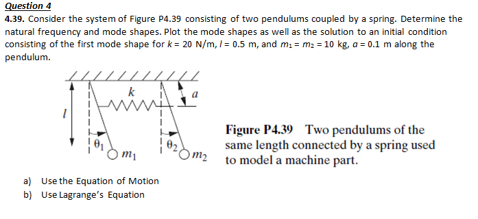 Question 4
4.39. Consider the system of Figure P4.39 consisting of two pendulums coupled by a spring. Determine the
natural frequency and mode shapes. Plot the mode shapes as well as the solution to an initial condition
consisting of the first mode shape for k= 20 N/m, I= 0.5 m, and m= mz =10 kg, a= 0.1 m along the
pendulum.
I kN Ya
1
VA I
i i -
i I Figure P439 Two pendulums of the
101 16, same length connected by a spring used
! om ! my .
2 to model a machine part.
a) Usethe Equation of Motion
b) Uselagrange’s Equation