 VIPSolutions
Please provide step by step answerc. Find the competitive equilibrium by leaving out the goods market in initial calculations. Then verify Walras Law by showing that the goods market clears. Draw diagrams which show the supply and demand curves for each of the markets and show the competitive equilibrium prices and allocations. Aggregate Capital Stock: K = 900, Aggregate Labor Supply: L = 400, Production Function: Y = K.5L.5, Consumption Function: C = 70 + .7Yd, Investment Function: | = 84-100r, Government Spending: G = 100, Tax Collections: T = 100. With this production function MPL(K,L) = 5K.5L-.5andMPK(K,L) = 5K ——
Question:
Please provide step by step answer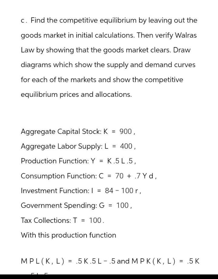 c. Find the competitive equilibrium by leaving out the
goods market in initial calculations. Then verify Walras
Law by showing that the goods market clears. Draw
diagrams which show the supply and demand curves
for each of the markets and show the competitive
equilibrium prices and allocations.
Aggregate Capital Stock: K = 900,
Aggregate Labor Supply: L = 400,
Production Function: Y = K.5L.5,
Consumption Function: C = 70 + .7Yd,
Investment Function: | = 84-100r,
Government Spending: G = 100,
Tax Collections: T = 100.
With this production function
MPL(K,L) = 5K.5L-.5andMPK(K,L) = 5K
——
This is AI generated Response.
Asked by: Vikram Kumar
Created at: 2025-09-24 01:24:05
Asked by: Vikram Kumar
Created at: 2025-09-24 01:24:05
Final Answer:
Rendered
Raw Text
Did you like this answer?
# Step-by-Step Solution
Let's break down the problem step by step:
---
## **1. Model Setup and Given Data**
- **Aggregate Capital (K):** 900
- **Aggregate Labor (L):** 400
- **Production Function:** \( Y = K^{0.5} L^{0.5} \)
- **Consumption Function:** \( C = 70 + 0.7Y_d \)
- **Investment Function:** \( I = 84 - 100r \)
- **Government Spending (G):** 100
- **Taxes (T):** 100
- **Marginal Products:**
- \( MPL = 0.5 K^{0.5} L^{-0.5} \)
- \( MPK = 0.5 K^{-0.5} L^{0.5} \)
---
## **2. Find Output (Y)**
Plug in \( K = 900 \), \( L = 400 \):
\[
Y = 900^{0.5} \times 400^{0.5} = 30 \times 20 = 600
\]
---
## **3. Find Factor Prices (Wage and Rental Rate)**
**Wage (\( w \)) = \( MPL \):**
\[
MPL = 0.5 \times 900^{0.5} \times 400^{-0.5} = 0.5 \times 30 \times \frac{1}{20} = 0.5 \times 1.5 = 0.75
\]
**Rental Rate (\( r \)) = \( MPK \):**
\[
MPK = 0.5 \times 900^{-0.5} \times 400^{0.5} = 0.5 \times \frac{1}{30} \times 20 = 0.5 \times 0.6667 = 0.3333
\]
---
## **4. Income and Disposable Income**
**Total Output (Income):** \( Y = 600 \)
**Taxes (T):** 100
**Disposable Income (\( Y_d \)):**
\[
Y_d = Y - T = 600 - 100 = 500
\]
---
## **5. Consumption (C):**
\[
C = 70 + 0.7 \times 500 = 70 + 350 = 420
\]
---
## **6. Investment (I):**
\[
I = 84 - 100r
\]
We don't know \( r \) yet; let's find equilibrium.
---
## **7. Goods Market Equilibrium**
\[
Y = C + I + G
\]
\[
600 = 420 + (84 - 100r) + 100
\]
\[
600 = 420 + 100 + 84 - 100r
\]
\[
600 = 604 - 100r
\]
\[
100r = 604 - 600 = 4
\]
\[
r = 0.04
\]
---
**Now plug \( r \) back into the Investment function:**
\[
I = 84 - 100 \times 0.04 = 84 - 4 = 80
\]
---
## **8. Verify Walras' Law (Goods Market Clears)**
\[
Y = C + I + G
\]
\[
600 = 420 + 80 + 100 = 600
\]
**Goods market clears.**
---
## **9. Competitive Equilibrium Summary**
| Variable | Value |
|----------|-------|
| Output (\( Y \)) | 600 |
| Consumption (\( C \)) | 420 |
| Investment (\( I \)) | 80 |
| Government Spending (\( G \)) | 100 |
| Taxes (\( T \)) | 100 |
| Wage (\( w \)) | 0.75 |
| Rental Rate (\( r \)) | 0.04 |
---
## **10. Market Diagrams (Sketch Description)**
**Labor Market:**
- **Supply:** Vertical at \( L = 400 \)
- **Demand:** Downward sloping from \( MPL \) as function of \( L \)
- **Equilibrium Wage:** \( w = 0.75 \)
**Capital Market:**
- **Supply:** Vertical at \( K = 900 \)
- **Demand:** Downward sloping from \( MPK \) as function of \( K \)
- **Equilibrium Rental Rate:** \( r = 0.04 \)
**Goods Market:**
- **Supply:** Horizontal at \( Y = 600 \)
- **Demand:** \( C + I + G = 600 \)
- **Equilibrium at \( Y = 600 \)**
---
## **11. Summary Table**
| Market | Supply | Demand | Equilibrium Price | Equilibrium Quantity |
|-------------|---------------|------------------|-------------------|---------------------|
| Labor | 400 | From \( MPL \) | \( w = 0.75 \) | 400 |
| Capital | 900 | From \( MPK \) | \( r = 0.04 \) | 900 |
| Goods | 600 | 600 | — | 600 |
---
### **Conclusion**
- **Equilibrium allocations:** \( Y = 600 \), \( L = 400 \), \( K = 900 \)
- **Equilibrium prices:** \( w = 0.75 \), \( r = 0.04 \)
- **Goods market clears, verifying Walras' Law.**
---
If you need hand-drawn diagrams, let me know and I can describe how to sketch them!
Question:
need hand-drawn diagrams,
This is AI generated Response.
Asked by: Vikram Kumar
Created at: 2025-09-24 01:25:42
Asked by: Vikram Kumar
Created at: 2025-09-24 01:25:42
Final Answer:
Rendered
Raw Text
Did you like this answer?
## Hand-Drawn Diagrams Description
### **1. Labor Market Diagram**
- **Axes:**
- X-axis: Quantity of Labor (L)
- Y-axis: Wage Rate (w)
- **Supply Curve:**
- Vertical line at \( L = 400 \) (perfectly inelastic supply).
- **Demand Curve:**
- Downward sloping from \( MPL \) values. Start high on the Y-axis and slope downwards toward the right.
- **Equilibrium Point:**
- Mark the intersection of the demand curve and the vertical supply line.
- Label equilibrium wage \( w = 0.75 \).
### **2. Capital Market Diagram**
- **Axes:**
- X-axis: Quantity of Capital (K)
- Y-axis: Rental Rate (r)
- **Supply Curve:**
- Vertical line at \( K = 900 \).
- **Demand Curve:**
- Downward sloping from \( MPK \) values. Start high on the Y-axis and slope downwards toward the right.
- **Equilibrium Point:**
- Mark the intersection of the demand curve and the vertical supply line.
- Label equilibrium rental rate \( r = 0.04 \).
### **3. Goods Market Diagram**
- **Axes:**
- X-axis: Total Output (Y)
- Y-axis: Aggregate Demand
- **Supply Curve:**
- Horizontal line at \( Y = 600 \) (perfectly elastic supply).
- **Demand Curve:**
- Downward sloping curve based on \( C + I + G \) values, intersecting the supply line at \( Y = 600 \).
- **Equilibrium Point:**
- Mark the intersection of the demand curve and the horizontal supply line.
- Label total output \( Y = 600 \).
### **Visual Elements to Include:**
- Use different colors for supply and demand curves.
- Clearly label axes, equilibrium points, and values.
- Add arrows to indicate the direction of shifts if needed.
---
This description provides a guide to creating hand-drawn diagrams for each market. If you need further details or modifications, please let me know!
📢 Instructions:
- Ask anything relatd to above question only.
- For new Question goto :