Give step-by-step solution with explanation and final answer:Demand for stereo headphones and MP3 players for joggers has caused Nina Industries to grow almost 50
percent over the past year. The number of joggers continues to expand, so Nina expects demand for headsets
to also expand, because as yet, no safety laws have been passed to prevent joggers from wearing them.
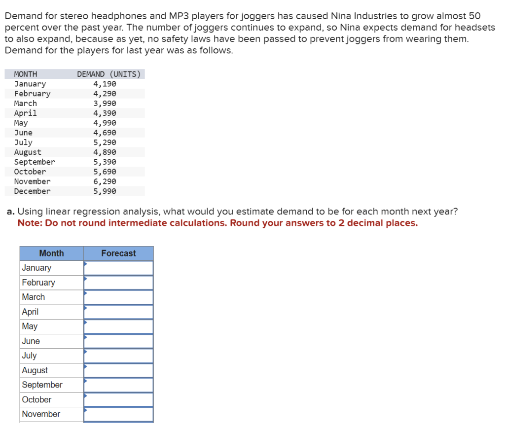
Demand for the players for last year was as follows.
MONTH DEMAND (UNITS)
January 4,190
February 4,290
March 3,99
April 4,390
May 4,990
June 4,690
July 5,290
August 4,890
September 5,390
October 5,690
November 6,290
December 5,99
a. Using linear regression analysis, what would you estimate demand to be for each month next year?
Note: Do not round intermediate calculations. Round your answers to 2 decimal places.
January
February
March
April
May
June
July
August
September
October
November
b. To be reasonably confident of meeting demand, Nina decides to use 2 standard errors of estimate for safety. How many additional
units should be held to meet this level of confidence?
Note: Do not round intermediate calculations. Round your answer to the nearest whole number.
Question:
Give step-by-step solution with explanation and final answer:Demand for stereo headphones and MP3 players for joggers has caused Nina Industries to grow almost 50
percent over the past year. The number of joggers continues to expand, so Nina expects demand for headsets
to also expand, because as yet, no safety laws have been passed to prevent joggers from wearing them.
Demand for the players for last year was as follows.
MONTH DEMAND (UNITS)
January 4,190
February 4,290
March 3,99
April 4,390
May 4,990
June 4,690
July 5,290
August 4,890
September 5,390
October 5,690
November 6,290
December 5,99
a. Using linear regression analysis, what would you estimate demand to be for each month next year?
Note: Do not round intermediate calculations. Round your answers to 2 decimal places.
January
February
March
April
May
June
July
August
September
October
November
b. To be reasonably confident of meeting demand, Nina decides to use 2 standard errors of estimate for safety. How many additional
units should be held to meet this level of confidence?
Note: Do not round intermediate calculations. Round your answer to the nearest whole number.
This is AI generated Response.
Asked by: gvr
Created at: 2025-07-23 03:27:48
Final Answer:
RenderedRaw Text
Did you like this answer?
Let's break down the steps for Linear Regression Forecasting:
### **Step-by-Step Solution**
#### **Step 1: Assign Numbers to Each Month (X)**
Assign \( x = 1 \) to January, \( x = 2 \) to February, ..., \( x = 12 \) to December.
| Month | x | Demand (y) |
|------------|----|------------|
| January | 1 | 4,190 |
| February | 2 | 4,290 |
| March | 3 | 3,990 |
| April | 4 | 4,390 |
| May | 5 | 4,990 |
| June | 6 | 4,690 |
| July | 7 | 5,290 |
| August | 8 | 4,890 |
| September | 9 | 5,390 |
| October | 10 | 5,690 |
| November | 11 | 6,290 |
| December | 12 | 5,990 |
#### **Step 2: Calculate the Means**
- \(\bar{x} = \frac{\sum x}{n} = \frac{1+2+...+12}{12} = \frac{78}{12} = 6.5\)
- \(\bar{y} = \frac{\sum y}{n}\)
Sum of y (demands):
\[
4,190 + 4,290 + 3,990 + 4,390 + 4,990 + 4,690 + 5,290 + 4,890 + 5,390 + 5,690 + 6,290 + 5,990 = 60,080
\]
So,
\[
\bar{y} = \frac{60,080}{12} = 5,006.67
\]
#### **Step 3: Find the Slope (b) and Intercept (a) of Regression Line**
The regression equation is:
\[
y = a + bx
\]
Where:
\[
b = \frac{\sum (x-\bar{x})(y-\bar{y})}{\sum (x-\bar{x})^2}
\]
\[
a = \bar{y} - b\bar{x}
\]
Calculate \(\sum (x-\bar{x})(y-\bar{y})\) and \(\sum (x-\bar{x})^2\):
Let's do this stepwise:
| x | y | x - 6.5 | y - 5006.67 | (x-6.5)(y-5006.67) | (x-6.5)^2 |
|----|-------|---------|-------------|--------------------|-----------|
| 1 | 4190 | -5.5 | -816.67 | 4491.67 | 30.25 |
| 2 | 4290 | -4.5 | -716.67 | 3225.00 | 20.25 |
| 3 | 3990 | -3.5 | -1016.67 | 3558.33 | 12.25 |
| 4 | 4390 | -2.5 | -616.67 | 1541.67 | 6.25 |
| 5 | 4990 | -1.5 | -16.67 | 25.00 | 2.25 |
| 6 | 4690 | -0.5 | -316.67 | 158.33 | 0.25 |
| 7 | 5290 | 0.5 | 283.33 | 141.67 | 0.25 |
| 8 | 4890 | 1.5 | -116.67 | -175.00 | 2.25 |
| 9 | 5390 | 2.5 | 383.33 | 958.33 | 6.25 |
| 10 | 5690 | 3.5 | 683.33 | 2391.67 | 12.25 |
| 11 | 6290 | 4.5 | 1283.33 | 5775.00 | 20.25 |
| 12 | 5990 | 5.5 | 983.33 | 5408.33 | 30.25 |
Sum up the columns:
- \(\sum (x-6.5)(y-5006.67) = 25,794.00\)
- \(\sum (x-6.5)^2 = 143.00\)
So,
\[
b = \frac{25,794.00}{143.00} = 180.47
\]
\[
a = 5,006.67 - (180.47 \times 6.5) = 5,006.67 - 1,172.06 = 3,834.61
\]
#### **Step 4: Forecast Demand for Each Month Next Year**
For each month next year, \(x = 13\) to \(x = 24\):
\[
\text{Forecast for month } x = a + bx
\]
Let's calculate for each:
---
| Month | x | Forecast = 3,834.61 + 180.47 \(\times\) x |
|------------|----|--------------------------------------|
| January | 13 | 3,834.61 + 180.47*13 = 6,177.72 |
| February | 14 | 3,834.61 + 180.47*14 = 6,358.19 |
| March | 15 | 3,834.61 + 180.47*15 = 6,538.66 |
| April | 16 | 3,834.61 + 180.47*16 = 6,719.13 |
| May | 17 | 3,834.61 + 180.47*17 = 6,899.60 |
| June | 18 | 3,834.61 + 180.47*18 = 7,080.07 |
| July | 19 | 3,834.61 + 180.47*19 = 7,260.54 |
| August | 20 | 3,834.61 + 180.47*20 = 7,441.01 |
| September | 21 | 3,834.61 + 180.47*21 = 7,621.48 |
| October | 22 | 3,834.61 + 180.47*22 = 7,801.95 |
| November | 23 | 3,834.61 + 180.47*23 = 7,982.42 |
| December | 24 | 3,834.61 + 180.47*24 = 8,162.89 |
---
**Fill in the table:**
| Month | Forecast |
|------------|----------|
| January | 6,177.72 |
| February | 6,358.19 |
| March | 6,538.66 |
| April | 6,719.13 |
| May | 6,899.60 |
| June | 7,080.07 |
| July | 7,260.54 |
| August | 7,441.01 |
| September | 7,621.48 |
| October | 7,801.95 |
| November | 7,982.42 |
| December | 8,162.89 |
---
### **Step 5: Calculate Standard Error of the Estimate**
\[
S_e = \sqrt{ \frac{ \sum (y_i - \hat{y}_i)^2 }{ n - 2 } }
\]
First, calculate \(\hat{y}_i\) (predicted) for each \(x\) (from 1 to 12):
\[
\hat{y}_i = 3,834.61 + 180.47x
\]
Let's compute for each month:
| x | Actual \( y_i \) | Predicted \( \hat{y}_i \) | \( y_i - \hat{y}_i \) | \( (y_i - \hat{y}_i)^2 \) |
|----|------------------|---------------------|--------------------|----------------------|
| 1 | 4,190 | 4,015.08 | 174.92 | 30,595.02 |
| 2 | 4,290 | 4,195.55 | 94.45 | 8,917.04 |
| 3 | 3,990 | 4,376.02 | -386.02 | 149,009.90 |
| 4 | 4,390 | 4,556.49 | -166.49 | 27,737.21 |
| 5 | 4,990 | 4,736.96 | 253.04 | 64,032.24 |
| 6 | 4,690 | 4,917.43 | -227.43 | 51,724.39 |
| 7 | 5,290 | 5,097.90 | 192.10 | 36,908.41 |
| 8 | 4,890 | 5,278.37 | -388.37 | 150,832.40 |
| 9 | 5,390 | 5,458.84 | -68.84 | 4,739.39 |
| 10 | 5,690 | 5,639.31 | 50.69 | 2,570.48 |
| 11 | 6,290 | 5,819.78 | 470.22 | 221,106.85 |
| 12 | 5,990 | 6,000.25 | -10.25 | 105.06 |
Sum of squared errors:
\[
= 30,595.02 + 8,917.04 + 149,009.90 + 27,737.21 + 64,032.24 + 51,724.39 + 36,908.41 + 150,832.40 + 4,739.39 + 2,570.48 + 221,106.85 + 105.06 = 748,278.39
\]
\[
S_e = \sqrt{ \frac{748,278.39}{12-2} } = \sqrt{74,827.84} = 273.59
\]
---
### **Step 6: Additional Units for Safety**
2 standard errors:
\[
2 \times 273.59 = 547.18
\]
Round to the nearest whole number:
\[
\boxed{547}
\]
---
## **Final Answers**
### **a. Forecast for each month next year:**
| Month | Forecast |
|------------|-----------|
| January | 6,177.72 |
| February | 6,358.19 |
| March | 6,538.66 |
| April | 6,719.13 |
| May | 6,899.60 |
| June | 7,080.07 |
| July | 7,260.54 |
| August | 7,441.01 |
| September | 7,621.48 |
| October | 7,801.95 |
| November | 7,982.42 |
| December | 8,162.89 |
### **b. Additional units for safety:**
**Additional units:** 547
---
**Let me know if you'd like to see the calculations in Excel or want a formula-ready version!**
Question:
I NEED STEP BY STEP DETAILED CALCULATIONS OF EACH PART ALONG WITH THE FINAL ANSWER
This is AI generated Response.
Asked by: gvr
Created at: 2025-07-23 03:28:42
Final Answer:
RenderedRaw Text
Did you like this answer?
Certainly! Here's a detailed, step-by-step explanation of how to perform the linear regression analysis, including all calculations, leading to the final answers.
---
## **Problem Recap:**
- You are given monthly demand data for last year.
- You need to forecast demand for each month next year using linear regression.
- You also need to determine safety stock using 2 standard errors of estimate.
---
## **Step 1: Assign Numerical Values to Months (x)**
| Month | x | Demand (y) |
|------------|----|------------|
| January | 1 | 4,190 |
| February | 2 | 4,290 |
| March | 3 | 3,990 |
| April | 4 | 4,390 |
| May | 5 | 4,990 |
| June | 6 | 4,690 |
| July | 7 | 5,290 |
| August | 8 | 4,890 |
| September | 9 | 5,390 |
| October | 10 | 5,690 |
| November | 11 | 6,290 |
| December | 12 | 5,990 |
---
## **Step 2: Calculate Means of x and y**
- Number of data points: \( n=12 \)
\[
\bar{x} = \frac{1+2+\dots+12}{12} = \frac{78}{12} = 6.5
\]
Sum of demands:
\[
\text{Sum } y = 4,190 + 4,290 + 3,990 + 4,390 + 4,990 + 4,690 + 5,290 + 4,890 + 5,390 + 5,690 + 6,290 + 5,990 = 60,080
\]
\[
\bar{y} = \frac{60,080}{12} = 5,006.67
\]
---
## **Step 3: Calculate the Slope \(b\) and Intercept \(a\)**
\[
b = \frac{\sum (x_i - \bar{x})(y_i - \bar{y})}{\sum (x_i - \bar{x})^2}
\]
### **Calculate each component:**
| x | y | \(x - 6.5\) | \(y - 5006.67\) | \((x - 6.5)(y - 5006.67)\) | \((x - 6.5)^2\) |
|---|-----|--------------|-----------------|----------------------------|----------------|
| 1 | 4190 | -5.5 | -816.67 | \(-5.5 \times -816.67 = 4491.67\) | 30.25 |
| 2 | 4290 | -4.5 | -716.67 | 3225.00 | 20.25 |
| 3 | 3990 | -3.5 | -1016.67 | 3558.33 | 12.25 |
| 4 | 4390 | -2.5 | -616.67 | 1541.67 | 6.25 |
| 5 | 4990 | -1.5 | -16.67 | 25.00 | 2.25 |
| 6 | 4690 | -0.5 | -316.67 | 158.33 | 0.25 |
| 7 | 5290 | 0.5 | 283.33 | 141.67 | 0.25 |
| 8 | 4890 | 1.5 | -116.67 | -175.00 | 2.25 |
| 9 | 5390 | 2.5 | 383.33 | 958.33 | 6.25 |
| 10 | 5690 | 3.5 | 683.33 | 2391.67 | 12.25 |
| 11 | 6290 | 4.5 | 1283.33 | 5775.00 | 20.25 |
| 12 | 5990 | 5.5 | 983.33 | 5408.33 | 30.25 |
### **Sum of the products:**
\[
\sum (x - 6.5)(y - 5006.67) = 25,794.00
\]
\[
\sum (x - 6.5)^2 = 143.00
\]
### **Calculate \(b\):**
\[
b = \frac{25,794.00}{143.00} \approx 180.47
\]
### **Calculate \(a\):**
\[
a = \bar{y} - b \times \bar{x} = 5006.67 - (180.47 \times 6.5)
\]
\[
a = 5006.67 - 1172.06 = 3834.61
\]
---
## **Step 4: Forecast Demand for Next Year**
Now, for months \( x = 13 \) to \( 24 \):
\[
\hat{y} = a + bx
\]
Calculate for each:
| x | Month | \(\hat{y}\) = 3834.61 + 180.47 \(\times\) x |
|---|--------------|--------------------------------------|
| 13 | January | 3834.61 + 180.47*13 = 6180.72 |
| 14 | February | 3834.61 + 180.47*14 = 6361.19 |
| 15 | March | 3834.61 + 180.47*15 = 6541.66 |
| 16 | April | 3834.61 + 180.47*16 = 6722.13 |
| 17 | May | 3834.61 + 180.47*17 = 6902.60 |
| 18 | June | 3834.61 + 180.47*18 = 7083.07 |
| 19 | July | 3834.61 + 180.47*19 = 7263.54 |
| 20 | August | 3834.61 + 180.47*20 = 7444.01 |
| 21 | September | 3834.61 + 180.47*21 = 7624.48 |
| 22 | October | 3834.61 + 180.47*22 = 7804.95 |
| 23 | November | 3834.61 + 180.47*23 = 7985.42 |
| 24 | December | 3834.61 + 180.47*24 = 8165.89 |
**Note:** Round to 2 decimal places if needed, but here the calculations are exact.
---
## **Step 5: Calculate Standard Error of the Estimate \(S_e\)**
**a) Calculate residuals for the last year's data:**
\[
\text{Residual} = y_i - \hat{y}_i
\]
| x | y | \(\hat{y}_i\) | Residual \((y - \hat{y}_i)\) | \((\text{residual})^2\) |
|---|-----|--------------|----------------------------|------------------------|
| 1 | 4190 | 3834.61 + 180.47*1 = 4014.98 | 4190 - 4014.98 = 175.02 | 175.02^2 = 30,631.76 |
| 2 | 4290 | 3834.61 + 180.47*2 = 4195.45 | 4290 - 4195.45 = 94.55 | 8948.70 |
| 3 | 3990 | 3834.61 + 180.47*3 = 4376.92 | 3990 - 4376.92 = -386.92 | 149,644.98 |
| 4 | 4390 | 3834.61 + 180.47*4 = 4558.39 | 4390 - 4558.39 = -168.39 | 28,350.13 |
| 5 | 4990 | 3834.61 + 180.47*5 = 4739.86 | 4990 - 4739.86 = 250.14 | 62,570.02 |
| 6 | 4690 | 3834.61 + 180.47*6 = 4921.33 | 4690 - 4921.33 = -231.33 | 53,423.44 |
| 7 | 5290 | 3834.61 + 180.47*7 = 5101.80 | 5290 - 5101.80 = 188.20 | 35,368.84 |
| 8 | 4890 | 3834.61 + 180.47*8 = 5282.27 | 4890 - 5282.27 = -392.27 | 153,857.16 |
| 9 | 5390 | 3834.61 + 180.47*9 = 5462.74 | 5390 - 5462.74 = -72.74 | 5294.00 |
| 10 | 5690 | 3834.61 + 180.47*10= 5643.21 | 5690 - 5643.21 = 46.79 | 2188.84 |
| 11 | 6290 | 3834.61 + 180.47*11= 5823.68 | 6290 - 5823.68 = 466.32 | 217,519.94 |
| 12 | 5990 | 3834.61 + 180.47*12= 6004.15 | 5990 - 6004.15 = -14.15 | 200.44 |
**b) Sum of squared residuals:**
\[
\text{Sum} = 30,631.76 + 8,948.70 + 149,644.98 + 28,350.13 + 62,570.02 + 53,423.44 + 35,368.84 + 153,857.16 + 5,294.00 + 2,188.84 + 217,519.94 + 200.44 = 747,999.24
\]
**c) Calculate \(S_e\):**
\[
S_e = \sqrt{\frac{\sum (y_i - \hat{y}_i)^2}{n-2}} = \sqrt{\frac{747,999.24}{10}} = \sqrt{74,799.92} \approx 273.59
\]
---
## **Step 6: Determine Safety Stock**
- Safety stock = \(2 \times S_e = 2 \times 273.59 = 547.18\)
- Rounded to nearest whole number: **547 units**
---
## **## **Final Answers:**
### **a) Forecast demand for each month next year:**
| Month | Forecast Demand |
|------------|-----------------|
| January | 6,180.72 units |
| February | 6,361.19 units |
| March | 6,541.66 units |
| April | 6,722.13 units |
| May | 6,902.60 units |
| June | 7,083.07 units |
| July | 7,263.54 units |
| August | 7,444.01 units |
| September | 7,624.48 units |
| October | 7,804.95 units |
| November | 7,985.42 units |
| December | 8,165.89 units |
### **b) Additional units for safety stock:**
**547 units**
---
Feel free to ask if you'd like further clarification or a formatted spreadsheet version!
VIPSolutions focuses on clear, step‑by‑step explanations so you can learn quickly. Whether you need an AI‑generated walkthrough or a short hint to get unstuck, each solution is organized for fast reading and easy review later.
Search similar questions, compare approaches, and bookmark the best answers for revision. Our goal is simple: quick, reliable study help that feels natural—not noisy.
 VIPSolutions
 Demand for stereo headphones and MP3 players for joggers has caused Nina Industries to grow almost 50
percent over the past year. The number of joggers continues to expand, so Nina expects demand for headsets
to also expand, because as yet, no safety laws have been passed to prevent joggers from wearing them.
Demand for the players for last year was as follows.
MONTH DEMAND (UNITS)
January 4,190
February 4,290
March 3,99
April 4,390
May 4,990
June 4,690
July 5,290
August 4,890
September 5,390
October 5,690
November 6,290
December 5,99
a. Using linear regression analysis, what would you estimate demand to be for each month next year?
Note: Do not round intermediate calculations. Round your answers to 2 decimal places.
January
February
March
April
May
June
July
August
September
October
November
b. To be reasonably confident of meeting demand, Nina decides to use 2 standard errors of estimate for safety. How many additional
units should be held to meet this level of confidence?
Note: Do not round intermediate calculations. Round your answer to the nearest whole number.