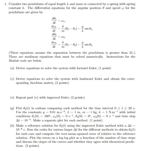
Give step-by-step solution with explanation and final answer:1. Consider two pendulums of equal length L and mass m connected by a spring with spring
constant k. The differential equations for the angular position 6 and specd w for the
pendulums are given by
a
= —
ky 6) Ian
or L-o)- Lune,
do
= —
dir ko 0
Ge —6)— Fsine,
(These equations assume the separation between the pendulums is greater than 2L.)
These are nonlinear equations that must be solved numerically. Instructions for the
Matlab code are below.
(a) Derive equations to solve the system with forward Euler; (1 point)
(€) Derive equations to solve the system with backward Euler and obtain the corre.
sponding Jacobian matrix; (2 points)
(€) Repeat part (c) with improved Euler; (2 points)
(2) Plot 6(¢) in radians comparing each method for the time interval 0 < t < 20 s.
Use the constants g = 981 ms, L = 1 m, m = 1 kg, k = 1 Nom? with initial
conditions 6,(0) = 160°, w;(0) = 05, 60) = 0°, w5(0) = 0 5°! and time step
At = 10". Make a separate plot for each method. (1 point)
(h) Make a reference solution for 6(t) using the improved Euler method with a At —
10% 5. Run the codes for various larger At for the different methods to obtain f(t)
for cach case and compute the root mean squared error of relative to the reference
solution. Plot the errors on a log log plot as a function of the mumber of time steps
and discuss the slopes of the curves and whether they agree with theoretical predic-
tions. (2 points)
Question:
Give step-by-step solution with explanation and final answer:1. Consider two pendulums of equal length L and mass m connected by a spring with spring
constant k. The differential equations for the angular position 6 and specd w for the
pendulums are given by
a
= —
ky 6) Ian
or L-o)- Lune,
do
= —
dir ko 0
Ge —6)— Fsine,
(These equations assume the separation between the pendulums is greater than 2L.)
These are nonlinear equations that must be solved numerically. Instructions for the
Matlab code are below.
(a) Derive equations to solve the system with forward Euler; (1 point)
(€) Derive equations to solve the system with backward Euler and obtain the corre.
sponding Jacobian matrix; (2 points)
(€) Repeat part (c) with improved Euler; (2 points)
(2) Plot 6(¢) in radians comparing each method for the time interval 0 < t < 20 s.
Use the constants g = 981 ms, L = 1 m, m = 1 kg, k = 1 Nom? with initial
conditions 6,(0) = 160°, w;(0) = 05, 60) = 0°, w5(0) = 0 5°! and time step
At = 10". Make a separate plot for each method. (1 point)
(h) Make a reference solution for 6(t) using the improved Euler method with a At —
10% 5. Run the codes for various larger At for the different methods to obtain f(t)
for cach case and compute the root mean squared error of relative to the reference
solution. Plot the errors on a log log plot as a function of the mumber of time steps
and discuss the slopes of the curves and whether they agree with theoretical predic-
tions. (2 points)
This is AI generated Response.
Asked by: gvr
Created at: 2025-07-09 08:17:17
Final Answer:
RenderedRaw Text
Did you like this answer?
Let's break down the solution step by step for each part mentioned in the problem statement:
---
## **Given System of Equations**
Let:
- \(\theta_1, \omega_1\): angular position and speed of pendulum 1
- \(\theta_2, \omega_2\): angular position and speed of pendulum 2
\[
\frac{d\theta_1}{dt} = \omega_1
\]
\[
\frac{d\omega_1}{dt} = \frac{k}{m}(\theta_2 - \theta_1) - \frac{g}{L}\sin\theta_1
\]
\[
\frac{d\theta_2}{dt} = \omega_2
\]
\[
\frac{d\omega_2}{dt} = \frac{k}{m}(\theta_1 - \theta_2) - \frac{g}{L}\sin\theta_2
\]
---
### **(a) Forward Euler Method**
Let \( \mathbf{y} = [\theta_1, \omega_1, \theta_2, \omega_2]^T \).
The general Forward Euler update is:
\[
\mathbf{y}_{n+1} = \mathbf{y}_n + \Delta t \cdot \mathbf{f}(\mathbf{y}_n)
\]
Where:
- \( \mathbf{f}(\mathbf{y}) \) is the right-hand side of the ODE system.
**Explicitly:**
\[
\theta_{1, n+1} = \theta_{1, n} + \Delta t \cdot \omega_{1, n}
\]
\[
\omega_{1, n+1} = \omega_{1, n} + \Delta t \left[\frac{k}{m}(\theta_{2, n} - \theta_{1, n}) - \frac{g}{L}\sin\theta_{1, n} \right]
\]
\[
\theta_{2, n+1} = \theta_{2, n} + \Delta t \cdot \omega_{2, n}
\]
\[
\omega_{2, n+1} = \omega_{2, n} + \Delta t \left[\frac{k}{m}(\theta_{1, n} - \theta_{2, n}) - \frac{g}{L}\sin\theta_{2, n} \right]
\]
---
### **(c) Backward Euler Method and Jacobian**
Backward Euler:
\[
\mathbf{y}_{n+1} = \mathbf{y}_n + \Delta t \cdot \mathbf{f}(\mathbf{y}_{n+1})
\]
You have to solve for \( \mathbf{y}_{n+1} \) implicitly (usually by Newton's method), so you need the Jacobian \( J = \frac{\partial \mathbf{f}}{\partial \mathbf{y}} \).
Let \( \mathbf{y} = [\theta_1, \omega_1, \theta_2, \omega_2]^T \):
\[
\mathbf{f}(\mathbf{y}) =
\begin{bmatrix}
\omega_1 \\
\frac{k}{m}(\theta_2 - \theta_1) - \frac{g}{L}\sin\theta_1 \\
\omega_2 \\
\frac{k}{m}(\theta_1 - \theta_2) - \frac{g}{L}\sin\theta_2
\end{bmatrix}
\]
**Jacobian matrix \( J \):**
\[
J =
\begin{bmatrix}
0 & 1 & 0 & 0 \\
-\frac{k}{m} - \frac{g}{L}\cos\theta_1 & 0 & \frac{k}{m} & 0 \\
0 & 0 & 0 & 1 \\
\frac{k}{m} & 0 & -\frac{k}{m} - \frac{g}{L}\cos\theta_2 & 0
\end{bmatrix}
\]
---
### **(e) Improved Euler (Heun's) Method**
Improved Euler (Heun's) method:
1. Predictor (Forward Euler): \( \mathbf{y}^* = \mathbf{y}_n + \Delta t \cdot \mathbf{f}(\mathbf{y}_n) \)
2. Corrector: \( \mathbf{y}_{n+1} = \mathbf{y}_n + \frac{\Delta t}{2} \left[\mathbf{f}(\mathbf{y}_n) + \mathbf{f}(\mathbf{y}^*)\right] \)
So, for this system, compute \( \mathbf{f}(\mathbf{y}_n) \), predict \( \mathbf{y}^* \), then average slopes.
---
### **(g) Plot \(\theta_2(t)\) for Each Method**
- Implement each method with given constants and initial conditions.
- Integrate from \( t=0 \) to \( t=20\,s \) with \( \Delta t = 10^{-3} \) s.
- Make separate plots for each integration method, showing \( \theta_2(t) \) (in radians).
---
### **(h) Reference Solution and Error Analysis**
- Compute a "reference" solution for \( \theta_2(t) \) using improved Euler with \( \Delta t = 10^{-6} \) s.
- For a range of larger \( \Delta t \), calculate the root-mean-square error (RMSE) for each method:
\[
\text{RMSE} = \sqrt{\frac{1}{N} \sum_{i=1}^{N} \left( \theta_{2,\text{num}}(t_i) - \theta_{2,\text{ref}}(t_i) \right)^2 }
\]
- Plot errors vs. number of steps (\( N = T/\Delta t \)) on a log-log scale for each method.
- Discuss slopes and agreement with theoretical convergence rates.
---
## **Final Answers Summary**
**(a) Forward Euler:**
\[
\boxed{
\begin{aligned}
\theta_{1, n+1} &= \theta_{1, n} + \Delta t \, \omega_{1, n} \\
\omega_{1, n+1} &= \omega_{1, n} + \Delta t \left[\frac{k}{m}(\theta_{2, n} - \theta_{1, n}) - \frac{g}{L}\sin\theta_{1, n}\right] \\
\theta_{2, n+1} &= \theta_{2, n} + \Delta t \, \omega_{2, n} \\
\omega_{2, n+1} &= \omega_{2, n} + \Delta t \left[\frac{k}{m}(\theta_{1, n} - \theta_{2, n}) - \frac{g}{L}\sin\theta_{2, n}\right]
\end{aligned}
}
\]
---
**(c) Backward Euler:**
\[
\boxed{
\begin{aligned}
\theta_{1, n+1} &= \theta_{1, n} + \Delta t \, \omega_{1, n+1} \\
\omega_{1, n+1} &= \omega_{1, n} + \Delta t \left[\frac{k}{m}(\theta_{2, n+1} - \theta_{1, n+1}) - \frac{g}{L}\sin\theta_{1, n+1}\right] \\
\theta_{2, n+1} &= \theta_{2, n} + \Delta t \, \omega_{2, n+1} \\
\omega_{2, n+1} &= \omega_{2, n} + \Delta t \left[\frac{k}{m}(\theta_{1, n+1} - \theta_{2, n+1}) - \frac{g}{L}\sin\theta_{2, n+1}\right]
\end{aligned}
}
\]
Jacobian given above.
---
**(e) Improved Euler (Heun's):**
1. Predictor: Use Forward Euler to get \( \mathbf{y}^* \).
2. Corrector:
\[
\mathbf{y}_{n+1} = \mathbf{y}_n + \frac{\Delta t}{2} \left[\mathbf{f}(\mathbf{y}_n) + \mathbf{f}(\mathbf{y}^*)\right]
\]
---
**(g,h) Plots and Error Analysis:**
- Plot \( \theta_2(t) \) for each method.
- For error analysis, plot RMSE vs. \( N \) (number of time steps) in log-log scale, and discuss convergence.
---
**If you need Matlab code or further details for each step, let me know!**
Question:
i need step by step detailed calculations of each part along with the final Answer
This is AI generated Response.
Asked by: gvr
Created at: 2025-07-09 08:19:11
Final Answer:
RenderedRaw Text
Did you like this answer?
Certainly! Here's a detailed step-by-step derivation and explanation for each part of the problem, along with the final formulas and how you can implement them.
---
## **Problem Restatement**
We have two pendulums connected by a spring, with equations:
\[
\frac{d\theta_1}{dt} = \omega_1
\]
\[
\frac{d\omega_1}{dt} = \frac{k}{m}(\theta_2 - \theta_1) - \frac{g}{L}\sin \theta_1
\]
\[
\frac{d\theta_2}{dt} = \omega_2
\]
\[
\frac{d\omega_2}{dt} = \frac{k}{m}(\theta_1 - \theta_2) - \frac{g}{L}\sin \theta_2
\]
with known parameters:
- \( g = 981\, \mathrm{m/s^2} \)
- \( L = 1\, \mathrm{m} \)
- \( m = 1\, \mathrm{kg} \)
- \( k = 1\, \mathrm{N/m} \)
Initial conditions:
- \( \theta_1(0) = 160^\circ \approx 2.7925\, \mathrm{rad} \)
- \( \omega_1(0) = 0.5\, \mathrm{rad/s} \)
- \( \theta_2(0) = 0^\circ = 0\, \mathrm{rad} \)
- \( \omega_2(0) = 0.5\, \mathrm{rad/s} \)
Time step:
- \( \Delta t = 10^{-3}\, \mathrm{s} \)
---
## **Part (a): Forward Euler Method**
### **Step 1: Write the system as a vector differential equation**
Define:
\[
\mathbf{y} =
\begin{bmatrix}
\theta_1 \\
\omega_1 \\
\theta_2 \\
\omega_2
\end{bmatrix}
\]
and
\[
\frac{d\mathbf{y}}{dt} = \mathbf{f}(\mathbf{y}) =
\begin{bmatrix}
\omega_1 \\
\frac{k}{m} (\theta_2 - \theta_1) - \frac{g}{L} \sin \theta_1 \\
\omega_2 \\
\frac{k}{m} (\theta_1 - \theta_2) - \frac{g}{L} \sin \theta_2
\end{bmatrix}
\]
### **Step 2: Forward Euler update formula**
\[
\mathbf{y}_{n+1} = \mathbf{y}_n + \Delta t \cdot \mathbf{f}(\mathbf{y}_n)
\]
which gives component-wise:
\[
\boxed{
\begin{aligned}
\theta_{1, n+1} &= \theta_{1, n} + \Delta t \, \omega_{1, n} \\
\omega_{1, n+1} &= \omega_{1, n} + \Delta t \left[ \frac{k}{m} (\theta_{2, n} - \theta_{1, n}) - \frac{g}{L} \sin \theta_{1, n} \right] \\
\theta_{2, n+1} &= \theta_{2, n} + \Delta t \, \omega_{2, n} \\
\omega_{2, n+1} &= \omega_{2, n} + \Delta t \left[ \frac{k}{m} (\theta_{1, n} - \theta_{2, n}) - \frac{g}{L} \sin \theta_{2, n} \right]
\end{aligned}
}
\]
---
## **Part (c): Backward Euler Method**
### **Step 1: Implicit scheme**
\[
\mathbf{y}_{n+1} = \mathbf{y}_n + \Delta t \cdot \mathbf{f}(\mathbf{y}_{n+1})
\]
This involves solving for \( \mathbf{y}_{n+1} \) because \( \mathbf{f} \) depends on \( \mathbf{y}_{n+1} \).
### **Step 2: Write the equations explicitly**
\[
\begin{cases}
\theta_{1, n+1} &= \theta_{1, n} + \Delta t \, \omega_{1, n+1} \\
\omega_{1, n+1} &= \omega_{1, n} + \Delta t \left[ \frac{k}{m} (\theta_{2, n+1} - \theta_{1, n+1}) - \frac{g}{L} \sin \theta_{1, n+1} \right] \\
\theta_{2, n+1} &= \theta_{2, n} + \Delta t \, \omega_{2, n+1} \\
\omega_{2, n+1} &= \omega_{2, n} + \Delta t \left[ \frac{k}{m} (\theta_{1, n+1} - \theta_{2, n+1}) - \frac{g}{L} \sin \theta_{2, n+1} \right]
\end{cases}
\]
### **Step 3: Solving implicitly**
This is a nonlinear system for \( \theta_{1, n+1}, \omega_{1, n+1}, \theta_{2, n+1}, \omega_{2, n+1} \). Typically, a Newton-Raphson iterative method is used:
- **Initial guess:** Use the previous step's values \( \mathbf{y}_n \).
- **Update:** Use the Jacobian matrix to get corrections until convergence.
### **Step 4: Jacobian matrix**
Define the residuals:
\[
\mathbf{R}(\mathbf{y}_{n+1}) = \mathbf{y}_{n+1} - \mathbf{y}_n - \Delta t \cdot \mathbf{f}(\mathbf{y}_{n+1}) = 0
\]
The Jacobian matrix \( J = \partial \mathbf{R} / \partial \mathbf{y}_{n+1} \), which is:
\[
J =
\begin{bmatrix}
1 & 0 & 0 & 0 \\
- \Delta t \frac{\partial f_2}{\partial \theta_1} & 1 - \Delta t \frac{\partial f_2}{\partial \omega_1} & - \Delta t \frac{\partial f_2}{\partial \theta_2} & - \Delta t \frac{\partial f_2}{\partial \omega_2} \\
0 & 0 & 1 & 0 \\
- \Delta t \frac{\partial f_4}{\partial \theta_1} & - \Delta t \frac{\partial f_4}{\partial \omega_1} & - \Delta t \frac{\partial f_4}{\partial \theta_2} & 1 - \Delta t \frac{\partial f_4}{\partial \omega_2}
\end{bmatrix}
\]
where:
\[
f_2 = \frac{k}{m} (\theta_2 - \theta_1) - \frac{g}{L} \sin \theta_1
\]
\[
f_4 = \frac{k}{m} (\theta_1 - \theta_2) - \frac{g}{L} \sin \theta_2
\]
Compute derivatives:
\[
\frac{\partial f_2}{\partial \theta_1} = - \frac{k}{m} - \frac{g}{L} \cos \theta_1
\]
\[
\frac{\partial f_2}{\partial \theta_2} = \frac{k}{m}
\]
\[
\frac{\partial f_2}{\partial \omega_1} = 0
\]
\[
\frac{\partial f_2}{\partial \omega_2} = 0
\]
Similarly for \( f_4 \):
\[
\frac{\partial f_4}{\partial \theta_1} = \frac{k}{m}
\]
\[
\frac{\partial f_4}{\partial \theta_2} = - \frac{k}{m} - \frac{g}{L} \cos \theta_2
\]
\[
\frac{\partial f_4}{\partial \omega_1} = 0
\]
\[
\frac{\partial f_4}{\partial \omega_2} = 0
\]
---
## **Part (e): Improved Euler (Heun's) Method**
### **Step 1: Compute the predictor**
\[
\mathbf{y}^* = \mathbf{y}_n + \Delta t \cdot \mathbf{f}(\mathbf{y}_n)
\]
### **Step 2: Compute the corrector**
\[
\mathbf{y}_{n+1} = \mathbf{y}_n + \frac{\Delta t}{2} \left[\mathbf{f}(\mathbf{y}_n) + \mathbf{f}(\mathbf{y}^*) \right]
\]
## **Summary**
---
## **Final expressions**
### **Forward Euler:**
\[
\boxed{
\begin{aligned}
\theta_{1, n+1} &= \theta_{1, n} + \Delta t \, \omega_{1, n} \\
\omega_{1, n+1} &= \omega_{1, n} + \Delta t \left[ \frac{k}{m} (\theta_{2, n} - \theta_{1, n}) - \frac{g}{L} \sin \theta_{1, n} \right] \\
\theta_{2, n+1} &= \theta_{2, n} + \Delta t \, \omega_{2, n} \\
\omega_{2, n+1} &= \omega_{2, n} + \Delta t \left[ \frac{k}{m} (\theta_{1, n} - \theta_{2, n}) - \frac{g}{L} \sin \theta_{2, n} \right]
\end{aligned}
}
\]
### **Backward Euler:**
\[
\boxed{
\text{Solve iteratively for } \mathbf{y}_{n+1} \text{ from:}
}
\]
\[
\begin{cases}
\theta_{1, n+1} &= \theta_{1, n} + \Delta t \, \omega_{1, n+1} \\
\omega_{1, n+1} &= \omega_{1, n} + \Delta t \left[ \frac{k}{m} (\theta_{2, n+1} - \theta_{1, n+1}) - \frac{g}{L} \sin \theta_{1, n+1} \right] \\
\theta_{2, n+1} &= \theta_{2, n} + \Delta t \, \omega_{2, n+1} \\
\omega_{2, n+1} &= \omega_{2, n} + \Delta t \left[ \frac{k}{m} (\theta_{1, n+1} - \theta_{2, n+1}) - \frac{g}{L} \sin \theta_{2, n+1} \right]
\end{cases}
\]
with Jacobian as derived.
### **Improved Euler (Heun):**
1. Predictor:
\[
\mathbf{y}^* = \mathbf{y}_n + \Delta t \, \mathbf{f}(\mathbf{y}_n)
\]
2. Corrector:
\[
\boxed{
\mathbf{y}_{n+1} = \mathbf{y}_n + \frac{\Delta t}{2} \left[ \mathbf{f}(\mathbf{y}_n) + \mathbf{f}(\mathbf{y}^*) \right]
}
\]
---
## **Next Steps**
- Implement these formulas in MATLAB or Python.
- Run simulations for each method.
- Plot \( \theta_2(t) \) over \( 0 < t < 20\,s \).
- Generate a reference solution with very small \( \Delta t \).
- Compute RMSE for larger \( \Delta t \) and plot errors.
---
If you'd like, I can also help you write the MATLAB code for each method or guide you through the implementation.
VIPSolutions focuses on clear, step‑by‑step explanations so you can learn quickly. Whether you need an AI‑generated walkthrough or a short hint to get unstuck, each solution is organized for fast reading and easy review later.
Search similar questions, compare approaches, and bookmark the best answers for revision. Our goal is simple: quick, reliable study help that feels natural—not noisy.
 VIPSolutions
 1. Consider two pendulums of equal length L and mass m connected by a spring with spring
constant k. The differential equations for the angular position 6 and specd w for the
pendulums are given by
a
= —
ky 6) Ian
or L-o)- Lune,
do
= —
dir ko 0
Ge —6)— Fsine,
(These equations assume the separation between the pendulums is greater than 2L.)
These are nonlinear equations that must be solved numerically. Instructions for the
Matlab code are below.
(a) Derive equations to solve the system with forward Euler; (1 point)
(€) Derive equations to solve the system with backward Euler and obtain the corre.
sponding Jacobian matrix; (2 points)
(€) Repeat part (c) with improved Euler; (2 points)
(2) Plot 6(¢) in radians comparing each method for the time interval 0 < t < 20 s.
Use the constants g = 981 ms, L = 1 m, m = 1 kg, k = 1 Nom? with initial
conditions 6,(0) = 160°, w;(0) = 05, 60) = 0°, w5(0) = 0 5°! and time step
At = 10". Make a separate plot for each method. (1 point)
(h) Make a reference solution for 6(t) using the improved Euler method with a At —
10% 5. Run the codes for various larger At for the different methods to obtain f(t)
for cach case and compute the root mean squared error of relative to the reference
solution. Plot the errors on a log log plot as a function of the mumber of time steps
and discuss the slopes of the curves and whether they agree with theoretical predic-
tions. (2 points)