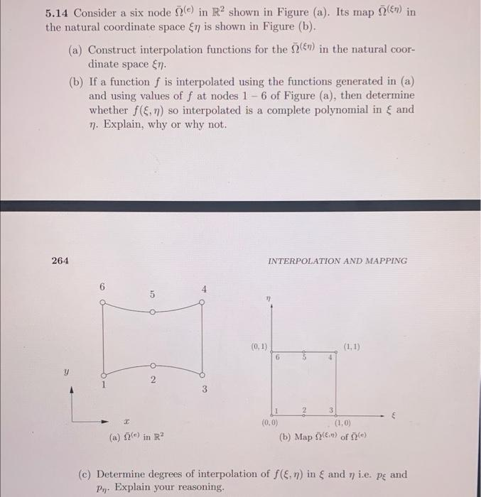
Give step-by-step solution with explanation and final answer:5.14 Consider a six node 2) in R* shown in Figure (a). Its map Q€7 in
the natural coordinate space €1 is shown in Figure (b).
(a) Construct interpolation functions for the 0€?) in the natural coor-
dinate space £1
(b) If a function f is interpolated using the functions generated in (a)
and using values of f at nodes 1 — 6 of Figure (a), then determine
whether f(€,7) so interpolated is a complete polynomial in £ and
7 Explain, why or why not
264 INTERPOLATION AND MAPPING
6 K i
|
| oy SW
u =2—4
1 2
[) 3
ia pe
V— =z 0,0) 0,0 V
(®) 8 in B? (6) Map OE of 0)
(¢) Determine degrees of interpolation of f(€.7) in § and 7 i.e. pe and
Py. Explain your reasoning.
Question:
Give step-by-step solution with explanation and final answer:5.14 Consider a six node 2) in R* shown in Figure (a). Its map Q€7 in
the natural coordinate space €1 is shown in Figure (b).
(a) Construct interpolation functions for the 0€?) in the natural coor-
dinate space £1
(b) If a function f is interpolated using the functions generated in (a)
and using values of f at nodes 1 — 6 of Figure (a), then determine
whether f(€,7) so interpolated is a complete polynomial in £ and
7 Explain, why or why not
264 INTERPOLATION AND MAPPING
6 K i
|
| oy SW
u =2—4
1 2
[) 3
ia pe
V— =z 0,0) 0,0 V
(®) 8 in B? (6) Map OE of 0)
(¢) Determine degrees of interpolation of f(€.7) in § and 7 i.e. pe and
Py. Explain your reasoning.
This is AI generated Response.
Asked by: gvr
Created at: 2025-06-30 03:41:15
Final Answer:
RenderedRaw Text
Did you like this answer?
Let's solve each part step by step:
---
**5.14 Consider a six-node element in \(\mathbb{R}^2\) shown in Figure (a). Its map in the natural coordinate space \(\xi \eta\) is shown in Figure (b).**
---
### (a) **Construct interpolation functions for the six-node element in the natural coordinate space \(\xi\eta\).**
#### **Step 1: Identify Nodes and Their Natural Coordinates**
From the diagram (b):
- Node 1: (0, 0)
- Node 2: (0.5, 0)
- Node 3: (1, 0)
- Node 4: (1, 1)
- Node 5: (0.5, 1)
- Node 6: (0, 1)
#### **Step 2: Quadratic Lagrange Interpolation Functions**
For a 6-node quadrilateral element, the standard shape functions in the natural coordinates \((\xi, \eta)\) are:
Let’s denote the nodes as follows:
- Corner nodes: 1, 3, 4, 6
- Midside nodes: 2, 5
The quadratic interpolation shape functions are:
\[
\begin{align*}
N_1(\xi, \eta) &= (1-\xi)(1-\eta)(-1+\xi+\eta)/4 \\
N_2(\xi, \eta) &= (1-\xi^2)(1-\eta)/2 \\
N_3(\xi, \eta) &= (1+\xi)(1-\eta)(-1-\xi+\eta)/4 \\
N_4(\xi, \eta) &= (1+\xi)(1+\eta)(-1-\xi-\eta)/4 \\
N_5(\xi, \eta) &= (1-\xi^2)(1+\eta)/2 \\
N_6(\xi, \eta) &= (1-\xi)(1+\eta)(-1+\xi-\eta)/4 \\
\end{align*}
\]
Alternatively, using the nodes at:
- \((\xi, \eta)\) = (0,0), (0.5,0), (1,0), (1,1), (0.5,1), (0,1)
The shape functions can be written using Lagrange polynomials:
- For \(\xi\): at 0, 0.5, 1
- For \(\eta\): at 0, 1
So:
- \(L_1(\xi) = (1-\xi)(1-2\xi)\) at \(\xi=0\)
- \(L_2(\xi) = 4\xi(1-\xi)\) at \(\xi=0.5\)
- \(L_3(\xi) = \xi(2\xi-1)\) at \(\xi=1\)
- \(M_1(\eta) = 1-\eta\) at \(\eta=0\)
- \(M_2(\eta) = \eta\) at \(\eta=1\)
Thus, the shape/interpolation functions are:
\[
\begin{align*}
N_1(\xi,\eta) &= L_1(\xi) M_1(\eta) = (1-\xi)(1-2\xi)(1-\eta) \\
N_2(\xi,\eta) &= L_2(\xi) M_1(\eta) = 4\xi(1-\xi)(1-\eta) \\
N_3(\xi,\eta) &= L_3(\xi) M_1(\eta) = \xi(2\xi-1)(1-\eta) \\
N_4(\xi,\eta) &= L_3(\xi) M_2(\eta) = \xi(2\xi-1)\eta \\
N_5(\xi,\eta) &= L_2(\xi) M_2(\eta) = 4\xi(1-\xi)\eta \\
N_6(\xi,\eta) &= L_1(\xi) M_2(\eta) = (1-\xi)(1-2\xi)\eta \\
\end{align*}
\]
---
### (b) **Is \(f(\xi, \eta)\) a complete polynomial in \(\xi\) and \(\eta\)?**
#### **Step 1: What is a "Complete Polynomial"?**
A complete polynomial of degree \(p\) in 2 variables contains all monomials up to degree \(p\):
- Degree 1: \(1, \xi, \eta\)
- Degree 2: \(1, \xi, \eta, \xi^2, \xi\eta, \eta^2\)
#### **Step 2: What does the 6-node interpolation produce?**
Look at the shape functions above: They include terms like \(\xi, \eta, \xi^2, \xi\eta\).
However, the interpolation is **quadratic in \(\xi\)** (since there are 3 points in \(\xi\): 0, 0.5, 1), but only **linear in \(\eta\)** (since there are only 2 distinct values: 0, 1).
Thus, **the interpolation is not a complete quadratic polynomial in both variables**—it is quadratic in \(\xi\) and linear in \(\eta\).
#### **Answer:**
> **No, \(f(\xi, \eta)\) interpolated using these functions is not a complete polynomial in \(\xi\) and \(\eta\).**
>
> It is quadratic in \(\xi\) and linear in \(\eta\), so not all terms up to degree 2 in both variables are present (e.g., there is no \(\eta^2\) term).
---
### (c) **Degrees of interpolation in \(\xi\) and \(\eta\), \(p_\xi\) and \(p_\eta\):**
- **In \(\xi\):** There are three nodes (0, 0.5, 1), so the interpolation is quadratic (\(p_\xi = 2\)).
- **In \(\eta\):** There are two nodes (0, 1), so the interpolation is linear (\(p_\eta = 1\)).
#### **Reasoning:**
The degree of interpolation is determined by the number of distinct nodes in each coordinate direction. Three points allow quadratic interpolation, two points allow linear interpolation.
---
## **Summary**
### **(a)**
The interpolation (shape) functions are:
\[
\begin{align*}
N_1(\xi,\eta) &= (1-\xi)(1-2\xi)(1-\eta) \\
N_2(\xi,\eta) &= 4\xi(1-\xi)(1-\eta) \\
N_3(\xi,\eta) &= \xi(2\xi-1)(1-\eta) \\
N_4(\xi,\eta) &= \xi(2\xi-1)\eta \\
N_5(\xi,\eta) &= 4\xi(1-\xi)\eta \\
N_6(\xi,\eta) &= (1-\xi)(1-2\xi)\eta \\
\end{align*}
\]
### **(b)**
No, \(f(\xi,\eta)\) is not a complete polynomial in \(\xi\) and \(\eta\), because the interpolation is quadratic in \(\xi\) and linear in \(\eta\).
### **(c)**
Degrees of interpolation: \(p_\xi = 2\), \(p_\eta = 1\).
---
**If you need further clarification or algebraic steps for the shape functions, let me know!**
Question:
i need part A detailed calculations along with the final Answer
This is AI generated Response.
Asked by: gvr
Created at: 2025-06-30 03:44:41
Final Answer:
RenderedRaw Text
Did you like this answer?
Let's proceed with a detailed, step-by-step calculation for **Part (a): Constructing the interpolation functions** for the six-node element in the natural coordinate space \((\xi, \eta)\).
---
### Step 1: Identify the Nodes and Their Natural Coordinates
From the diagram (Figure b), the six nodes are located at:
| Node | \(\xi\) | \(\eta\) |
|---------|---------|---------|
| 1 | 0 | 0 |
| 2 | 0.5 | 0 |
| 3 | 1 | 0 |
| 4 | 1 | 1 |
| 5 | 0.5 | 1 |
| 6 | 0 | 1 |
---
### Step 2: Recognize the Type of Element and Shape Functions
This is a **six-node (quadratic) quadrilateral element** with nodes at the corners and midpoints of sides.
The shape functions are constructed such that:
\[
f(\xi, \eta) = \sum_{i=1}^6 N_i(\xi, \eta) f_i
\]
where \(N_i(\xi, \eta)\) are the shape functions associated with nodes \(i\), satisfying:
\[
N_i(\xi_j, \eta_j) = \delta_{ij}
\]
---
### Step 3: Define the Interpolation Functions
Since the element is quadratic, the shape functions \(N_i(\xi, \eta)\) are quadratic polynomials in \(\xi\) and \(\eta\). They can be written as products of **Lagrange polynomials** in each coordinate:
\[
N_i(\xi, \eta) = L_{i,\xi}(\xi) \times L_{i,\eta}(\eta)
\]
---
### Step 4: Construct Lagrange Polynomials in \(\xi\) and \(\eta\)
For \(\xi\):
- Nodes at \(\xi = 0, 0.5, 1\)
Lagrange basis functions in \(\xi\):
\[
\begin{aligned}
l_0(\xi) &= \frac{(\xi - 0.5)(\xi - 1)}{(0 - 0.5)(0 - 1)} = \frac{(\xi - 0.5)(\xi - 1)}{(-0.5)(-1)} = \frac{(\xi - 0.5)(\xi - 1)}{0.5} \\
l_{0.5}(\xi) &= \frac{(\xi - 0)(\xi - 1)}{(0.5 - 0)(0.5 - 1)} = \frac{\xi (\xi - 1)}{(0.5)(-0.5)} = \frac{\xi (\xi - 1)}{-0.25} \\
l_1(\xi) &= \frac{(\xi - 0)(\xi - 0.5)}{(1 - 0)(1 - 0.5)} = \frac{\xi (\xi - 0.5)}{(1)(0.5)} = 2 \xi (\xi - 0.5) \\
\end{aligned}
\]
Similarly for \(\eta\):
- Nodes at \(\eta = 0, 1\)
Lagrange basis functions:
\[
\begin{aligned}
m_0(\eta) &= 1 - \eta \\
m_1(\eta) &= \eta \\
\end{aligned}
\]
---
### Step 5: Write the Shape Functions \(N_i(\xi, \eta)\)
Using the above basis functions, the shape functions are:
| Node | \(\xi_i, \eta_i\) | Shape Function \(N_i(\xi,\eta)\) |
|---------|-------------------|----------------------------------|
| 1 | (0, 0) | \(N_1 = l_0(\xi) \times m_0(\eta)\) |
| 2 | (0.5, 0) | \(N_2 = l_{0.5}(\xi) \times m_0(\eta)\) |
| 3 | (1, 0) | \(N_3 = l_1(\xi) \times m_0(\eta)\) |
| 4 | (1, 1) | \(N_4 = l_1(\xi) \times m_1(\eta)\) |
| 5 | (0.5, 1) | \(N_5 = l_{0.5}(\xi) \times m_1(\eta)\) |
| 6 | (0, 1) | \(N_6 = l_0(\xi) \times m_1(\eta)\) |
---
### **Explicit Forms of \(l_0(\xi), l_{0.5}(\xi), l_1(\xi)\):**
\[
\boxed{
\begin{aligned}
l_0(\xi) &= \frac{(\xi - 0.5)(\xi - 1)}{0.5} = 2 (\xi - 0.5)(\xi - 1) \\
l_{0.5}(\xi) &= \frac{\xi (\xi - 1)}{-0.25} = -4 \xi (\xi - 1) \\
l_1(\xi) &= 2 \xi (\xi - 0.5) \\
\end{aligned}
}
\]
Similarly:
\[
\boxed{
\begin{aligned}
m_0(\eta) &= 1 - \eta \\
m_1(\eta) &= \eta \\
\end{aligned}
}
\]
---
### **Final Expressions for the Six Shape Functions:**
\[
\boxed{
\begin{aligned}
N_1(\xi, \eta) &= l_0(\xi) \times m_0(\eta) = 2 (\xi - 0.5)(\xi - 1) \times (1 - \eta) \\
N_2(\xi, \eta) &= l_{0.5}(\xi) \times m_0(\eta) = -4 \xi (\xi - 1) \times (1 - \eta) \\
N_3(\xi, \eta) &= l_1(\xi) \times m_0(\eta) = 2 \xi (\xi - 0.5) \times (1 - \eta) \\
N_4(\xi, \eta) &= l_1(\xi) \times m_1(\eta) = 2 \xi (\xi - 0.5) \times \eta \\
N_5(\xi, \eta) &= l_{0.5}(\xi) \times m_1(\eta) = -4 \xi (\xi - 1) \times \eta \\
N_6(\xi, \eta) &= l_0(\xi) \times m_1(\eta) = 2 (\xi - 0.5)(\xi - 1) \times \eta \\
\end{aligned}
}
\]
---
### **Summary of Part (a):**
The **interpolation functions** (shape functions) for the six-node quadratic element in natural coordinates \((\xi, \eta)\) are:
\[
\boxed{
\begin{aligned}
\boxed{
N_1(\xi, \eta) = 2 (\xi - 0.5)(\xi - 1) (1 - \eta)
}
}
\quad
\boxed{
N_2(\xi, \eta) = -4 \xi (\xi - 1) (1 - \eta)
}
\quad
\boxed{
N_3(\xi, \eta) = 2 \xi (\xi - 0.5) (1 - \eta)
}
\]
\[
\boxed{
N_4(\xi, \eta) = 2 \xi (\xi - 0.5) \eta
}
\quad
\boxed{
N_5(\xi, \eta) = -4 \xi (\xi - 1) \eta
}
\quad
\boxed{
N_6(\xi, \eta) = 2 (\xi - 0.5)(\xi - 1) \eta
}
\]
---
**This completes the detailed solution for Part (a).** If you'd like, I can help with further parts or clarify the derivation.
VIPSolutions focuses on clear, step‑by‑step explanations so you can learn quickly. Whether you need an AI‑generated walkthrough or a short hint to get unstuck, each solution is organized for fast reading and easy review later.
Search similar questions, compare approaches, and bookmark the best answers for revision. Our goal is simple: quick, reliable study help that feels natural—not noisy.
 VIPSolutions
 5.14 Consider a six node 2) in R* shown in Figure (a). Its map Q€7 in
the natural coordinate space €1 is shown in Figure (b).
(a) Construct interpolation functions for the 0€?) in the natural coor-
dinate space £1
(b) If a function f is interpolated using the functions generated in (a)
and using values of f at nodes 1 — 6 of Figure (a), then determine
whether f(€,7) so interpolated is a complete polynomial in £ and
7 Explain, why or why not
264 INTERPOLATION AND MAPPING
6 K i
|
| oy SW
u =2—4
1 2
[) 3
ia pe
V— =z 0,0) 0,0 V
(®) 8 in B? (6) Map OE of 0)
(¢) Determine degrees of interpolation of f(€.7) in § and 7 i.e. pe and
Py. Explain your reasoning.