 VIPSolutions
Give step-by-step solution with explanation and final answer:Question 4: 20 Marks. Consider the mel » FT TP+14P% where P(t) represents the size of the population at time £. 1) Tots logistic modet? sity your answer (42) Draw a phase line of the model, (43) Draw a sketch of the solution curve P(t), if P(0) = 7. Question. 14 Marks sume tha for the sysm Ee) oc. a graph of the function G looks like this: S X “1 05 2 (5.1) Draw a rough graph of what the function G(x) could look like. (52) Draw a rough sketch of the solution curves x(t) when the initial value is x(0) = 1 and when the initial value is x(0) = 0.
Question:
Give step-by-step solution with explanation and final answer: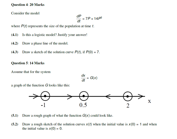 Question 4: 20 Marks.
Consider the mel »
FT TP+14P%
where P(t) represents the size of the population at time £.
1) Tots logistic modet? sity your answer
(42) Draw a phase line of the model,
(43) Draw a sketch of the solution curve P(t), if P(0) = 7.
Question. 14 Marks
sume tha for the sysm
Ee)
oc.
a graph of the function G looks like this:
S X
“1 05 2
(5.1) Draw a rough graph of what the function G(x) could look like.
(52) Draw a rough sketch of the solution curves x(t) when the initial value is x(0) = 1 and when
the initial value is x(0) = 0.
This is AI generated Response.
Asked by: gvr
Created at: 2025-07-15 08:34:54
Asked by: gvr
Created at: 2025-07-15 08:34:54
Final Answer:
Rendered
Raw Text
Did you like this answer?
Let's work through each part step-by-step:
---
## **Question 4**
Given:
\[
\frac{dP}{dt} = 7P + 14P^2
\]
### **(4.1) Is this a logistic model? Justify your answer!**
**Logistic model:**
A standard logistic model has the form:
\[
\frac{dP}{dt} = rP\left(1 - \frac{P}{K}\right)
\]
where \( r \) is the growth rate and \( K \) is the carrying capacity.
**Given model:**
\[
\frac{dP}{dt} = 7P + 14P^2 = 7P(1 + 2P)
\]
- This is NOT a logistic model because:
- The logistic model has a **negative quadratic term** (\(-P^2\)), which leads to a carrying capacity.
- Here, the quadratic term is **positive** (\(+14P^2\)), which means the population will grow **faster** as \(P\) increases, and there is **no limiting value or carrying capacity**.
- Thus, the population grows without bound (super-exponential growth).
**Final answer:**
> **No, this is not a logistic model. In a logistic model, the quadratic term is negative to represent a carrying capacity that limits growth, but here the quadratic term is positive, leading to unbounded growth.**
---
### **(4.2) Draw a phase line of the model**
The phase line is based on the sign of \( \frac{dP}{dt} \):
\[
\frac{dP}{dt} = 7P + 14P^2 = 7P(1 + 2P)
\]
- Equilibrium points: Set \( \frac{dP}{dt} = 0 \):
- \( 7P = 0 \implies P = 0 \)
- \( 1 + 2P = 0 \implies P = -\frac{1}{2} \)
- Test intervals:
- For \( P < -\frac{1}{2} \): both factors negative and positive → \( \frac{dP}{dt} > 0 \)
- For \( -\frac{1}{2} < P < 0 \): first factor negative, second positive → \( \frac{dP}{dt} < 0 \)
- For \( P > 0 \): both factors positive → \( \frac{dP}{dt} > 0 \)
**Phase line:**
```
P: -∞ -----> -1/2 <----- 0 -----> ∞
(↑) (↓) (↑)
```
---
### **(4.3) Draw a sketch of the solution curve \( P(t) \), if \( P(0) = 7 \).**
- Since \( P(0) = 7 > 0 \):
- From the phase line, for \( P > 0 \), \( \frac{dP}{dt} > 0 \) so \( P(t) \) increases.
- The growth is faster than exponential (super-exponential, "blow-up" in finite time).
- The curve will rise steeply and go to infinity in finite time.
**Sketch:**
- Start at \( P = 7 \) at \( t = 0 \).
- Rapidly rises, curving upwards more and more steeply.
---
## **Question 5**
Given the phase line for \( \frac{dx}{dt} = G(x) \):
Arrows:
\( x < -1 \): right
\( -1 < x < 0.5 \): right
\( 0.5 < x < 2 \): left
\( x > 2 \): left
Equilibrium points: at \( x = -1, 0.5, 2 \)
### **(5.1) Draw a rough graph of what the function \( G(x) \) could look like.**
- \( G(x) = 0 \) at \( x = -1, 0.5, 2 \)
- \( G(x) > 0 \) where arrows are right (i.e., \( x < 0.5 \))
- \( G(x) < 0 \) where arrows are left (i.e., \( x > 0.5 \))
**Rough graph:**
```
G(x)
↑
|
| o o o
| / \ / \ / \
|-------|---|--|---|--|---|----> x
-1 0.5 2
```
- A possible sketch: G(x) positive between \( -\infty \) and \( 0.5 \), negative between \( 0.5 \) and \( \infty \), touching zero at the equilibrium points.
---
### **(5.2) Draw a rough sketch of the solution curves \( x(t) \) for:**
- \( x(0) = 1 \)
- \( x(0) = 0 \)
**For \( x(0) = 1 \):**
- \( 0.5 < 1 < 2 \), so arrows point left, \( x \) decreases toward \( x = 0.5 \).
**For \( x(0) = 0 \):**
- \( -1 < 0 < 0.5 \), so arrows point right, \( x \) increases toward \( x = 0.5 \).
**Sketch:**
- Both solutions approach \( x = 0.5 \) as \( t \to \infty \).
- \( x(t) \) increases from 0 to 0.5.
- \( x(t) \) decreases from 1 to 0.5.
---
## **Summary Table**
| Question | Step | Answer/Explanation |
|----------|------|-------------------|
| 4.1 | | No, not logistic; positive quadratic term. |
| 4.2 | | Phase line: Equilibria at \( P = 0, -0.5 \), arrows →, ←, →. |
| 4.3 | | \( P(t) \) for \( P(0)=7 \) grows rapidly, blows up in finite time. |
| 5.1 | | \( G(x) \) positive below 0.5 (zero at -1, 0.5), negative above 0.5 (zero at 2) |
| 5.2 | | Both \( x(0)=1 \) and \( x(0)=0 \) approach \( x=0.5 \) as \( t \to \infty \) |
---
Do you want the sketches/graphs drawn out? Let me know!
Question:
i need step by step detailed calculations of each part along with the final Answer
This is AI generated Response.
Asked by: gvr
Created at: 2025-07-15 08:39:31
Asked by: gvr
Created at: 2025-07-15 08:39:31
Final Answer:
Rendered
Raw Text
Did you like this answer?
Certainly! Let's proceed with each part step-by-step, providing detailed calculations, reasoning, and final answers.
---
## **Question 4**
Given differential equation:
\[
\frac{dP}{dt} = 7P + 14P^2
\]
---
### **(4.1) Is this a logistic model? Justify your answer**
**Step 1:** Recall the standard logistic model:
\[
\frac{dP}{dt} = r P \left( 1 - \frac{P}{K} \right)
\]
which expands to:
\[
\frac{dP}{dt} = r P - \frac{r P^2}{K}
\]
with:
- **Linear term:** \( r P \)
- **Quadratic term:** \( - \frac{r}{K} P^2 \) (negative quadratic)
**Step 2:** Compare with the given model:
\[
\frac{dP}{dt} = 7 P + 14 P^2
\]
- The quadratic term here is **positive** (\(+14 P^2\)).
**Step 3:** **Implication of quadratic term sign:**
- In logistic growth, the quadratic term is negative, which models a **limiting effect** (carrying capacity).
- Here, the quadratic term is positive, implying **accelerated growth** with no limiting population—super-exponential growth.
**Final conclusion:**
\[
\boxed{
\text{No, this is not a logistic model because the quadratic term is positive, indicating unbounded growth.}
}
\]
---
### **(4.2) Draw a phase line for the model**
**Step 1:** Find equilibrium points where \(\frac{dP}{dt} = 0\):
\[
7P + 14P^2 = 0
\]
Factor out \(7P\):
\[
7P (1 + 2P) = 0
\]
So,
\[
P = 0 \quad \text{or} \quad 1 + 2P = 0 \implies P = -\frac{1}{2}
\]
**Step 2:** Sign analysis of \(\frac{dP}{dt}\):
- For \(P < -\frac{1}{2}\):
- \(P\) negative, \(1 + 2P\) negative \(\Rightarrow\) \(7P\) negative, \(1+2P\) negative
- Product: negative \(\times\) negative = **positive**, so \(\frac{dP}{dt} > 0\).
- For \(-\frac{1}{2} < P < 0\):
- \(P\) negative, \(1 + 2P\) positive (since \(2P > -1\))
- Product: negative \(\times\) positive = **negative**, so \(\frac{dP}{dt} < 0\).
- For \(P > 0\):
- \(P\) positive, \(1 + 2P\) positive
- Product: positive \(\times\) positive = **positive**, so \(\frac{dP}{dt} > 0\).
**Step 3:** Sketch the phase line:
```
P: --------------|--------------|----------------
-∞ -1/2 0 +∞
Direction of \(\frac{dP}{dt}\):
- For \(P < -1/2\): + (arrow to the right)
- For \(-1/2 < P < 0\): - (arrow to the left)
- For \(P > 0\): + (arrow to the right)
Equilibria at \(P = -\frac{1}{2}\) and \(P= 0\).
```
**Optional:** Indicate stability:
- Near \(P = -\frac{1}{2}\):
- For \(P\) just less than \(-\frac{1}{2}\), \(\frac{dP}{dt} > 0\): solutions move away from \(-\frac{1}{2}\) to the left.
- For \(P\) just greater than \(-\frac{1}{2}\), \(\frac{dP}{dt} < 0\): solutions move toward \(-\frac{1}{2}\).
**Thus:** \(P = -\frac{1}{2}\) is **stable**.
- Near \(P=0\):
- For \(P\) just less than 0, \(\frac{dP}{dt} < 0\), solutions move toward 0.
- For \(P\) just greater than 0, \(\frac{dP}{dt} > 0\), solutions move away from 0.
**Thus:** \(P=0\) is **unstable**.
---
### **(4.3) Sketch the solution curve \( P(t) \) with \( P(0) = 7 \).**
**Step 1:** Initial condition:
\[
P(0) = 7 > 0
\]
- From the phase line, for \(P > 0\), \(\frac{dP}{dt} > 0\), **population increases**.
**Step 2:** Behavior:
- Since \(\frac{dP}{dt} = 7 P + 14 P^2\), for large \(P\), the quadratic term dominates, and the growth accelerates rapidly.
- The solution "blows-up" (becomes infinite) in **finite time** because the differential equation resembles a super-exponential growth.
**Step 3:** Qualitative sketch:
- The curve starts at \(P=7\) at \(t=0\).
- As \(t\) increases, \(P(t)\) increases rapidly, becoming steeper.
- Approaching some finite time \(T\), \(P(t) \to +\infty\).
**Final note:**
- The solution is **not bounded** and exhibits **finite-time blow-up**.
---
## **Summary for Question 4:**
| Part | Explanation | Final Answer |
|--------|--------------|--------------|
| 4.1 | Comparing with logistic form; quadratic term positive | **No**, not logistic |
| 4.2 | Sign analysis of \(\frac{dP}{dt}\); equilibria at \(P=-1/2, 0\) | **Phase line**: stable at \(-1/2\), unstable at 0 |
| 4.3 | Behavior of \(P(t)\) for \(P(0)=7\) | Rapid, unbounded growth, blow-up in finite time |
---
## **Question 5**
Given the phase line arrows:
- \(x < -1\): right
- \(-1 < x < 0.5\): right
- \(0.5 < x < 2\): left
- \(x > 2\): left
Equilibria at \(x = -1, 0.5, 2\).
---
### **(5.1) Draw a rough graph of \( G(x) \).**
**Step 1:** Zeroes at \(x = -1, 0.5, 2\).
**Step 2:** Sign of \(G(x)\):
- To the **left of \(-1\)** (\(x < -1\)): \(G(x) > 0\), solutions move right.
- Between \(-1\) and \(0.5\): \(G(x) > 0\), solutions move right.
- Between \(0.5\) and \(2\): \(G(x) < 0\), solutions move left.
- To the **right of \(2\)**: \(G(x) < 0\), solutions move left.
**Step 3:** Sketch:
- \(G(x)\) crosses zero at the equilibrium points.
- Positive between \(-1\) and \(0.5\), negative between \(0.5\) and \(2\), zero at the equilibrium points.
**Final sketch:**
```
G(x)
↑
|
| / \ / \
|-------|---|------|---|------> x
-1 0.5 2
```
- The graph dips below zero between \(0.5\) and \(2\), crosses zero at the equilibrium points, and remains positive elsewhere.
---
### **(5.2) Sketch of solution curves \(x(t)\) for**
- \(x(0) = 1\)
- \(x(0) = 0\)
**Behavior analysis:**
- At \(x=1\): \(0.5 < 1 < 2\), so \(G(x) < 0\), solutions **decrease** toward \(x=0.5\).
- At \(x=0\): \(-1 < 0 < 0.5\), so \(G(x) > 0\), solutions **increase** toward \(x=0.5\).
**Final solution behavior:**
- Both initial points tend toward the stable equilibrium at \(x=0.5\).
**Sketch:**
- \(x(t)\) starting at 1 decreases toward 0.5.
- \(x(t)\) starting at 0 increases toward 0.5.
---
## **Summary for Question 5:**
| Part | Explanation | Final Answer |
|--------|--------------|--------------|
| 5.1 | \(G(x)\) crosses zero at \(-1, 0.5, 2\), positive and negative regions as per phase line | Graph crosses at these points, positive before \(-1\) and between \(-1, 0.5\), negative between \(0.5, 2\), negative after 2 |
| 5.2 | \(x(0)=1\) decreases toward 0.5; \(x(0)=0\) increases toward 0.5 | Both approach \(x=0.5\) as \(t \to \infty\) |
---
**Note:** For actual sketches, plotting with approximate curves showing zero crossings and direction arrows would help visualize the phase line and solution trajectories.
---
**If you'd like, I can generate the approximate sketches or further elaborate on the solution behavior.**
Question:
i need only final Answers of each part
This is AI generated Response.
Asked by: gvr
Created at: 2025-07-15 08:40:46
Asked by: gvr
Created at: 2025-07-15 08:40:46
Final Answer:
Rendered
Raw Text
Did you like this answer?
Certainly! Here are the final concise answers for each part:
---
### **Question 4**
**(4.1)**
**Answer:** No, this is not a logistic model because the quadratic term is positive, leading to unbounded (super-exponential) growth.
**(4.2)**
**Answer:** Equilibria at \( P = -\frac{1}{2} \) (stable) and \( P=0 \) (unstable). Phase line:
- \( P < -\frac{1}{2} \): \( \frac{dP}{dt} > 0 \) (arrow right)
- \(-\frac{1}{2} < P < 0 \): \( \frac{dP}{dt} < 0 \) (arrow left)
- \( P > 0 \): \( \frac{dP}{dt} > 0 \) (arrow right)
**(4.3)**
**Answer:** For initial \( P(0)=7 \), the solution \( P(t) \) increases rapidly and blows up to infinity in finite time.
---
### **Question 5**
**(5.1)**
**Answer:** \( G(x) \) has zeros at \( x = -1, 0.5, 2 \). It is positive on \((-\infty, -1)\) and \((-1, 0.5)\), negative on \((0.5, 2)\), and negative beyond \( 2 \).
**(5.2)**
**Answer:** The solutions starting at \( x=1 \) (between 0.5 and 2) decrease toward \( x=0.5 \); those starting at \( x=0 \) increase toward \( x=0.5 \). Both tend toward the stable equilibrium at \( x=0.5 \).
---
📢 Instructions:
- Ask anything relatd to above question only.
- For new Question goto :