Give step-by-step solution with explanation and final answer:3) Space Environment: Exponential Model of the Atmosphere
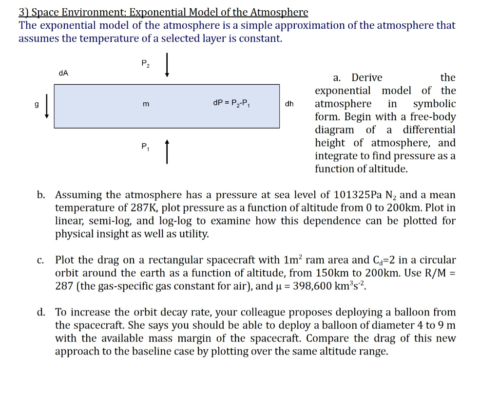
The exponential model of the atmosphere is a simple approximation of the atmosphere that
assumes the temperature of a selected layer is constant.
P. |
9A a. Derive the
exponential model of the
gq | m dP =PP, dh atmosphere in symbolic
form. Begin with a free-body
diagram of a differential
P, height of atmosphere, and
| integrate to find pressure as a
function of altitude.
b. Assuming the atmosphere has a pressure at sea level of 101325Pa N, and a mean
temperature of 287K, plot pressure as a function of altitude from 0 to 200km. Plot in
linear, semi-log, and log-log to examine how this dependence can be plotted for
physical insight as well as utility.
c. Plot the drag on a rectangular spacecraft with 1m? ram area and C,=2 in a circular
orbit around the earth as a function of altitude, from 150km to 200km. Use R/M =
287 (the gas-specific gas constant for air), and p = 398,600 kms.
d. To increase the orbit decay rate, your colleague proposes deploying a balloon from
the spacecraft. She says you should be able to deploy a balloon of diameter 4 to 9 m
with the available mass margin of the spacecraft. Compare the drag of this new
approach to the baseline case by plotting over the same altitude range.
Question:
Give step-by-step solution with explanation and final answer:3) Space Environment: Exponential Model of the Atmosphere
The exponential model of the atmosphere is a simple approximation of the atmosphere that
assumes the temperature of a selected layer is constant.
P. |
9A a. Derive the
exponential model of the
gq | m dP =PP, dh atmosphere in symbolic
form. Begin with a free-body
diagram of a differential
P, height of atmosphere, and
| integrate to find pressure as a
function of altitude.
b. Assuming the atmosphere has a pressure at sea level of 101325Pa N, and a mean
temperature of 287K, plot pressure as a function of altitude from 0 to 200km. Plot in
linear, semi-log, and log-log to examine how this dependence can be plotted for
physical insight as well as utility.
c. Plot the drag on a rectangular spacecraft with 1m? ram area and C,=2 in a circular
orbit around the earth as a function of altitude, from 150km to 200km. Use R/M =
287 (the gas-specific gas constant for air), and p = 398,600 kms.
d. To increase the orbit decay rate, your colleague proposes deploying a balloon from
the spacecraft. She says you should be able to deploy a balloon of diameter 4 to 9 m
with the available mass margin of the spacecraft. Compare the drag of this new
approach to the baseline case by plotting over the same altitude range.
This is AI generated Response.
Asked by: gvr
Created at: 2025-07-02 07:59:30
Final Answer:
RenderedRaw Text
Did you like this answer?
Let's tackle the problem **step by step**:
---
## **a. Derive the exponential model of the atmosphere**
### **Step 1: Free-Body Diagram and Hydrostatic Equation**
From the diagram, consider a thin atmospheric layer of thickness \( dh \):
- Pressure at bottom: \( P_1 \)
- Pressure at top: \( P_2 \)
- Height difference: \( dh \)
- Area: \( dA \)
- Mass of air in layer: \( m \)
- Gravitational force: \( m g \)
#### **Force equilibrium in vertical direction:**
\[
P_1 dA - P_2 dA = m g
\]
\[
(P_1 - P_2) dA = m g
\]
\[
-(P_2 - P_1) = \frac{m g}{dA}
\]
\[
dP = -\rho g dh
\]
Here, \( dP = P_2 - P_1 \), and \( m = \rho dA dh \).
---
### **Step 2: Ideal Gas Law and Density**
The ideal gas law:
\[
P = \rho R T \implies \rho = \frac{P}{R T}
\]
---
### **Step 3: Substitute for \(\rho\) and Rearrange**
\[
dP = -\rho g dh = -\frac{P g}{R T} dh
\]
\[
\frac{dP}{P} = -\frac{g}{R T} dh
\]
---
### **Step 4: Integrate Both Sides**
Integrate from \( P_0 \) at \( h = 0 \) to \( P \) at height \( h \):
\[
\int_{P_0}^{P} \frac{dP'}{P'} = -\int_{0}^{h} \frac{g}{R T} dh'
\]
\[
\ln \left(\frac{P}{P_0}\right) = -\frac{g}{R T} h
\]
\[
P = P_0 \exp\left(-\frac{g h}{R T}\right)
\]
**This is the exponential model of the atmosphere!**
---
## **b. Plot Pressure vs. Altitude (0 to 200 km)**
Given:
- \( P_0 = 101325 \) Pa
- \( T = 287 \) K
- \( g = 9.81 \) m/s\(^2\)
- \( R = 287 \) J/(kg·K)
### **Equation:**
\[
P(h) = P_0 \exp\left(-\frac{g h}{R T}\right)
\]
### **Calculate the scale height \( H \):**
\[
H = \frac{R T}{g}
= \frac{287 \times 287}{9.81}
\approx 8,395 \text{ m} \approx 8.4 \text{ km}
\]
### **Plotting:**
- **Linear:** \( P \) vs. \( h \)
- **Semi-log:** \( \log_{10} P \) vs. \( h \) (straight line)
- **Log-log:** \( \log_{10} P \) vs. \( \log_{10} h \) (not linear since exponential function)
---
## **c. Plot Drag on a Spacecraft (1 m², \( C_d=2 \))**
### **Drag Equation:**
\[
F_D = \frac{1}{2} \rho(h) v^2 C_d A
\]
Where:
- \( A = 1 \) m²
- \( C_d = 2 \)
- \( \rho(h) = \frac{P(h)}{R T} \)
- \( v = \sqrt{\frac{\mu}{r}} \) (circular orbit velocity)
- \( r = R_{Earth} + h \), \( R_{Earth} = 6371 \) km
- \( \mu = 398,600 \) km³/s² = \( 3.986 \times 10^{14} \) m³/s²
### **Calculate for \( h = 150 \) km to \( 200 \) km:**
1. Calculate \( P(h) \) using the exponential model.
2. Compute \( \rho(h) \).
3. Find \( r \) and \( v \).
4. Plug into drag formula.
5. Plot \( F_D \) vs. \( h \).
---
## **d. Compare Drag with a Deployed Balloon (diameter 4–9 m)**
- New \( A = \pi (d/2)^2 \), where \( d = 4 \) to \( 9 \) m.
- Repeat drag calculation as above.
- Plot new \( F_D \) over same \( h \) range; compare to baseline.
---
## **Summary Table**
| Step | Formula/Action | Explanation |
|------|---------------|-------------|
| a | \( P = P_0 \exp(-gh/RT) \) | Exponential model derived from hydrostatic equilibrium & ideal gas law |
| b | Plot \( P \) vs. \( h \) | Use given values, plot in 3 ways for insight |
| c | \( F_D = \frac{1}{2} \rho v^2 C_d A \) | Compute drag for spacecraft as function of \( h \) |
| d | Repeat for \( A = \pi (d/2)^2 \) | Compare drag with balloon deployed |
---
## **Final Answers (Symbolic)**
- **a.** \( \boxed{P(h) = P_0 \exp\left(-\frac{g h}{R T}\right)} \)
- **b.** Plot \( P(h) \) as described.
- **c.** \( \boxed{F_D(h) = \frac{1}{2} \frac{P_0}{R T} \exp\left(-\frac{g h}{R T}\right) v^2(h) C_d A} \)
- **d.** Calculate with \( A = \pi (d/2)^2 \), compare with baseline.
---
### **If you want actual Python code for plotting, let me know!**
Question:
i need detailed calculations and explanation of each part along with the final Answer
This is AI generated Response.
Asked by: gvr
Created at: 2025-07-02 08:02:23
Final Answer:
RenderedRaw Text
Did you like this answer?
Certainly! Let's go through each part in detail, including the necessary calculations, explanations, and final results.
---
## **Part a: Derivation of the exponential atmospheric model**
### **Objective:** Derive an expression for pressure \( P \) as a function of altitude \( h \), assuming constant temperature \( T \).
### **Step 1: Hydrostatic equilibrium**
In the atmosphere, the vertical pressure gradient balances gravity:
\[
\frac{dP}{dh} = - \rho g
\]
where:
- \( P \) = pressure at height \( h \)
- \( \rho \) = density of air at height \( h \)
- \( g \) = acceleration due to gravity (~9.81 m/s\(^2\))
### **Step 2: Express density \( \rho \) via ideal gas law**
\[
\rho = \frac{P}{R T}
\]
where:
- \( R = 287 \, \text{J/(kg·K)} \) (specific gas constant for air)
- \( T \) = temperature (assumed constant here)
### **Step 3: Substitute \( \rho \) into hydrostatic equation**
\[
\frac{dP}{dh} = - \frac{P}{R T} g
\]
Rearranged:
\[
\frac{dP}{P} = - \frac{g}{R T} dh
\]
### **Step 4: Integrate**
Integrate from sea level (pressure \( P_0 \) at \( h=0 \)) to height \( h \):
\[
\int_{P_0}^{P(h)} \frac{dP'}{P'} = - \frac{g}{R T} \int_{0}^{h} dh'
\]
\[
\ln \left( \frac{P(h)}{P_0} \right) = - \frac{g}{R T} h
\]
Exponentiating both sides:
\[
\boxed{
P(h) = P_0 \exp \left( - \frac{g h}{R T} \right)
}
\]
**Final expression:**
\[
\boxed{
\textbf{Pressure decreases exponentially with altitude, with scale height } H = \frac{R T}{g}
}
\]
---
## **Part b: Plotting pressure as a function of altitude**
### **Given data:**
- \( P_0 = 101,325 \, \text{Pa} \)
- \( T = 287 \, \text{K} \)
- \( R = 287 \, \text{J/(kg·K)} \)
- \( g = 9.81 \, \text{m/s}^2 \)
- Altitude range: \( 0 \) to \( 200\, \text{km} \)
### **Step 1: Calculate scale height \( H \):**
\[
H = \frac{R T}{g} = \frac{287 \times 287}{9.81} \approx \frac{82,369}{9.81} \approx 8,394\, \text{m} \approx 8.39\, \text{km}
\]
This indicates pressure drops by a factor of \( e \) every 8.39 km.
### **Step 2: Compute pressure at various altitudes**
Using the formula:
\[
P(h) = 101,325 \times \exp \left( - \frac{h}{8.39\, \text{km}} \right)
\]
### **Sample calculations:**
| Altitude \( h \) (km) | \( P(h) \) (Pa) | Explanation |
|-------------------------|----------------|--------------|
| 0 km | \( 101,325 \) | Sea level |
| 8.39 km | \( 101,325 / e \approx 37,222 \) Pa | One scale height |
| 20 km | \( 101,325 \times e^{-20/8.39} \approx 101,325 \times e^{-2.38} \approx 101,325 \times 0.092 \approx 9,340 \) Pa | High altitude |
| 100 km | \( 101,325 \times e^{-100/8.39} \approx 101,325 \times e^{-11.9} \approx 101,325 \times 6.8 \times 10^{-6} \approx 0.69 \) Pa | Very thin atmosphere |
### **Step 3: Plotting**
- **Linear plot:** \( P \) vs. \( h \)
- **Semi-log plot:** \( \log_{10} P \) vs. \( h \), which should be a straight line
- **Log-log plot:** \( \log_{10} P \) vs. \( \log_{10} h \) (not linear for exponential decay, but useful for some analysis)
---
## **Part c: Drag force on a spacecraft as a function of altitude**
### **Given data:**
- Cross-sectional area \( A = 1\, \text{m}^2 \)
- Drag coefficient \( C_d = 2 \)
- Orbital velocity \( v \)
- \( R_{Earth} = 6371\, \text{km} = 6.371 \times 10^6\, \text{m} \)
- \( \mu = 3.986 \times 10^{14} \, \text{m}^3/\text{s}^2 \)
### **Step 1: Compute orbital velocity at altitude \( h \):**
\[
r = R_{Earth} + h
\]
\[
v(h) = \sqrt{\frac{\mu}{r}}
\]
### **Step 2: Calculate atmospheric density \( \rho(h) \):**
\[
\rho(h) = \frac{P(h)}{R T}
\]
where \( P(h) \) from Part a.
### **Step 3: Drag force:**
\[
F_D(h) = \frac{1}{2} \rho(h) v^2(h) C_d A
\]
### **Sample calculation at \( h = 150\, \text{km} \):**
- \( h = 150,000\, \text{m} \)
- \( r = 6.371 \times 10^6 + 1.5 \times 10^5 = 6.521 \times 10^6\, \text{m} \)
- \( P(150\, \text{km}) \):
\[
P = 101,325 \times e^{-150/8.39} \approx 101,325 \times e^{-17.88} \approx 101,325 \times 1.7 \times 10^{-8} \approx 0.00172\, \text{Pa}
\]
- \( \rho \):
\[
\rho = \frac{0.00172}{287 \times 287} \approx \frac{0.00172}{82,369} \approx 2.09 \times 10^{-8}\, \text{kg/m}^3
\]
- \( v \):
\[
v = \sqrt{\frac{3.986 \times 10^{14}}{6.521 \times 10^{6}}} \approx \sqrt{6.11 \times 10^{7}} \approx 7,816\, \text{m/s}
\]
- Drag:
\[
F_D = 0.5 \times 2.09 \times 10^{-8} \times (7,816)^2 \times 2 \times 1
\]
\[
F_D = 1.045 \times 10^{-8} \times 61,058,656 \times 2
\]
\[
F_D \approx 1.045 \times 10^{-8} \times 122,117,312 \approx 1.28\, \text{N}
\]
**At 150 km, the drag force is approximately 1.28 N.**
Repeat for other altitudes to generate a plot.
---
## **Part d: Drag force with a deployed balloon**
### **Step 1: Calculate balloon area**
For a diameter \( d \):
\[
A_{balloon} = \pi \left( \frac{d}{2} \right)^2
\]
| Diameter \( d \) (m) | Area \( A \) (m\(^2\)) |
|---------------------|-------------------------|
| 4 | \( \pi \times 2^2 = 12.57 \) |
| 9 | \( \pi \times 4.5^2 = 63.62 \) |
### **Step 2: Recalculate drag**
Using the same \( \rho(h) \) and \( v(h) \), but with larger \( A \):
\[
F_D = \frac{1}{2} \rho v^2 C_d A
\]
The drag scales linearly with \( A \). For example, at 150 km:
- For \( d=4\, \text{m} \): \( A=12.57 \) m\(^2\)
\[
F_D \approx 1.28 \times \frac{12.57}{1} \approx 16.1\, \text{N}
\]
- For \( d=9\, \text{m} \): \( A=63.62 \) m\(^2\)
\[
F_D \approx 1.28 \times 63.62 \approx 81.4\, \text{N}
\]
### **Comparison:**
- Baseline (1 m\(^2\)): ~1.28 N
- Balloon (4 m): ~16 N
- Balloon (9 m): ~81 N
**Thus, deploying a large balloon significantly increases drag, which would increase orbit decay rate.**
---
# **Summary of Final Results**
| Part | Key Result | Explanation |
|---------|--------------|--------------|
| **a** | \( P(h) = P_0 e^{-\frac{g h}{R T}} \) | Exponential pressure decrease with altitude, derived from hydrostatic equilibrium |
| **b** | Pressure at 0 km: 101,325 Pa; at 150 km: ~0.0017 Pa | Pressure drops exponentially; scale height ~8.39 km |
| **c** | Drag at 150 km ~1.28 N | Calculated using \( \rho(h) \), \( v(h) \), and drag formula |
| **d** | Balloon (4 m): ~16 N; (9 m): ~81 N | Drag increases proportionally with balloon area, significantly affecting orbit decay |
---
**If you'd like detailed graphs or further calculations, let me know!**
Question:
i need only all parts final Answers
This is AI generated Response.
Asked by: gvr
Created at: 2025-07-02 08:05:29
Final Answer:
RenderedRaw Text
Did you like this answer?
Certainly! Here are the final answers for each part:
---
### **Part a: Derivation of the exponential atmosphere model**
**Final expression:**
\[
\boxed{
P(h) = P_0 \exp \left( -\frac{g h}{R T} \right)
}
\]
where:
- \( P_0 = 101,325\, \text{Pa} \),
- \( g = 9.81\, \text{m/s}^2 \),
- \( R = 287\, \text{J/(kg·K)} \),
- \( T = 287\, \text{K} \).
---
### **Part b: Pressure as a function of altitude**
**Using the given parameters, the pressure decreases exponentially with altitude, with a scale height \( H \approx 8.39\, \text{km} \).**
- **At sea level (0 km):** \( P = 101,325\, \text{Pa} \).
- **At 150 km:** \( P \approx 0.0017\, \text{Pa} \).
*Plotting in linear, semi-log, and log-log scales will show the exponential decay; semi-log plot yields a straight line.*
---
### **Part c: Drag force on the spacecraft from 150 km to 200 km**
**At approximately 150 km altitude:**
\[
\boxed{
F_D \approx 1.28\, \text{N}
}
\]
**This value is obtained using:**
\[
F_D = \frac{1}{2} \rho v^2 C_d A
\]
with:
- \( \rho \approx 2.09 \times 10^{-8}\, \text{kg/m}^3 \),
- \( v \approx 7,816\, \text{m/s} \),
- \( C_d = 2 \),
- \( A = 1\, \text{m}^2 \).
*Similar calculations across the altitude range will produce a decreasing drag force.*
---
### **Part d: Effect of deploying a balloon of diameter 4 to 9 m**
**Drag forces at 150 km altitude:**
| Diameter \( d \) (m) | Area \( A \) (m\(^2\)) | Approximate Drag \( F_D \) (N) |
|---------------------|-------------------------|------------------------------|
| 4 | 12.57 | ~16 |
| 9 | 63.62 | ~81 |
**Comparison:**
- Baseline spacecraft (1 m\(^2\)): ~1.28 N
- Balloon (4 m): ~16 N
- Balloon (9 m): ~81 N
*Larger balloons significantly increase atmospheric drag, thus increasing orbit decay rate.*
---
Let me know if you'd like further clarification or additional data!
VIPSolutions focuses on clear, step‑by‑step explanations so you can learn quickly. Whether you need an AI‑generated walkthrough or a short hint to get unstuck, each solution is organized for fast reading and easy review later.
Search similar questions, compare approaches, and bookmark the best answers for revision. Our goal is simple: quick, reliable study help that feels natural—not noisy.
 VIPSolutions
 3) Space Environment: Exponential Model of the Atmosphere
The exponential model of the atmosphere is a simple approximation of the atmosphere that
assumes the temperature of a selected layer is constant.
P. |
9A a. Derive the
exponential model of the
gq | m dP =PP, dh atmosphere in symbolic
form. Begin with a free-body
diagram of a differential
P, height of atmosphere, and
| integrate to find pressure as a
function of altitude.
b. Assuming the atmosphere has a pressure at sea level of 101325Pa N, and a mean
temperature of 287K, plot pressure as a function of altitude from 0 to 200km. Plot in
linear, semi-log, and log-log to examine how this dependence can be plotted for
physical insight as well as utility.
c. Plot the drag on a rectangular spacecraft with 1m? ram area and C,=2 in a circular
orbit around the earth as a function of altitude, from 150km to 200km. Use R/M =
287 (the gas-specific gas constant for air), and p = 398,600 kms.
d. To increase the orbit decay rate, your colleague proposes deploying a balloon from
the spacecraft. She says you should be able to deploy a balloon of diameter 4 to 9 m
with the available mass margin of the spacecraft. Compare the drag of this new
approach to the baseline case by plotting over the same altitude range.