 VIPSolutions
Give step-by-step solution with explanation and final answer:Problem Set 5 (Production Functions and Cost Minimization) 1. A firm has a production function given by F(K, L) = K*L* (a) For which values of a and 3 wil this function be constant returns to scale? For which will it be increasing or decreasing? (Hint: your answer will depend on the sum of a and 7). (b) Find the marginal product of capital and labor. For which values of a and 3 does the firm have diminishing marginal productivity of capital and labor? (
Question:
Give step-by-step solution with explanation and final answer: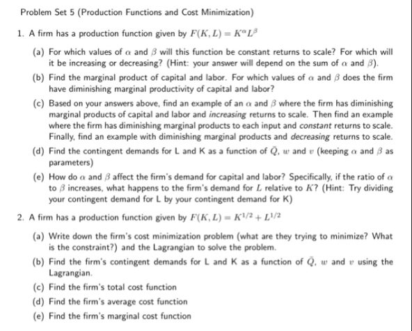 Problem Set 5 (Production Functions and Cost Minimization)
1. A firm has a production function given by F(K, L) = K*L*
(a) For which values of a and 3 wil this function be constant returns to scale? For which will
it be increasing or decreasing? (Hint: your answer will depend on the sum of a and 7).
(b) Find the marginal product of capital and labor. For which values of a and 3 does the firm
have diminishing marginal productivity of capital and labor?
(
This is AI generated Response.
Asked by: Vikram Kumar
Created at: 2025-11-15 04:02:22
Asked by: Vikram Kumar
Created at: 2025-11-15 04:02:22
Final Answer:
Rendered
Raw Text
Did you like this answer?
Let's solve each part step-by-step.
---
# **1. Production Function: \( F(K, L) = K^\alpha L^\beta \)**
## **(a) Returns to Scale**
- **Returns to scale:** Examine \( FK, t) = (K)^\ (tL^\beta = t^{\alphabeta} Kalpha L^\beta \)
- **If \( \alpha+\beta = 1 \):** Constant returns to scale
- **If \( \alpha+\beta > 1 \):** Increasing returns to scale
- **If \( \alpha+\beta < 1 \):** Decreasing returns to scale
---
## **(b) Marginal Products and Diminishing Marginal Product**
- **Marginal Product of Capital (MPK):**
\[
MP_K = \frac{\partial F}{\partial K} = \alpha K^{\alpha-1} L^\beta
\]
- **Marginal Product of Labor (MPL):**
\[
MP_L = \frac{\partial F}{\partial L} = \beta K^\alpha L^{\beta-1}
\]
- **Diminishing marginal product:** The second derivative w.r.t. each input should be negative.
- For capital:
\[
\frac{\partial^2 F}{\partial K^2} = \alpha(\alpha-1)K^{\alpha-2}L^\beta
\]
Diminishing if \( \alpha < 1 \).
- For labor:
\[
\frac{\partial^2 F}{\partial L^2} = \beta(\beta-1)K^\alpha L^{\beta-2}
\]
Diminishing if \( \beta < 1 \).
---
## **(c) Examples**
- **Diminishing marginal products, increasing returns to scale:** \( \alpha < 1, \beta < 1, \alpha+\beta > 1 \)
- **Diminishing marginal products, constant returns:** \( \alpha < 1, \beta < 1, \alpha+\beta = 1 \)
- **Diminishing marginal products, decreasing returns:** \( \alpha < 1, \beta < 1, \alpha+\beta < 1 \)
---
## **(d) Contingent Demands (Cost Minimization)**
Minimize cost \( C = wL + rK \) s.t. \( Q = K^\alpha L^\beta \):
Set up the Lagrangian:
\[
\mathcal{L} = wL + rK + \lambda(Q - K^\alpha L^\beta)
\]
First-order conditions:
- \( \frac{\partial \mathcal{L}}{\partial K} = r - \lambda \alpha K^{\alpha-1} L^\beta = \)
- \( \frac{\partial \mathcal{L}}{\partial L} = w - \lambda \beta K^\alpha L^{\beta-1} = \)
- \( \frac{\partial \mathcal{L}}{\partial \lambda} = Q - K^\alpha L^\beta = \)
Solve for \( K \) and \( L \):
Divide FOCs:
\[
\frac{r}{w} = \frac{\alpha}{\beta} \cdot \frac{L}{K}
\implies \frac{L}{K} = \frac{r\beta}{w\alpha}
\implies L = K \frac{r\beta}{w\alpha}
\]
Substitute into constraint:
\[
Q = K^\alpha \left(K \frac{r\beta}{w\alpha}\right)^\beta
= K^{\alpha+\beta} \left(\frac{r\beta}{w\alpha}\right)^\beta
\]
\[
K = Q^{\frac{1}{\alpha+\beta}} \left(\frac{w\alpha}{r\beta}\right)^{\frac{\beta}{\alpha+\beta}}
\]
\[
L = Q^{\frac{1}{\alpha+\beta}} \left(\frac{w\alpha}{r\beta}\right)^{\frac{\beta}{\alpha+\beta}} \frac{r\beta}{w\alpha}
= Q^{\frac{1}{\alpha+\beta}} \left(\frac{w\alpha}{r\beta}\right)^{\frac{\beta-1}{\alpha+\beta}} \left(\frac{r\beta}{w\alpha}\right)
\]
---
## **(e) Effect of \( \alpha \) and \( \beta \) on Demand for Inputs**
- If \( \frac{\alpha}{\beta} \) increases (i.e., alpha increases relative to beta), from above:
\[
\frac{L}{K} = \frac{r\beta}{w\alpha}
\]
- As \( \frac{\alpha}{\beta} \) increases, \( \frac{L}{K} \) **decreases**. So, **demand for labor relative to capital falls**.
---
# **2. Production Function: \( F(K, L) = K^{1/2} + L^{1/2} \)**
## **(a) Cost Minimization Problem**
- **Objective:** Minimize \( C = wL + rK \)
- **Constraint:** \( Q = K^{1/2} + L^{1/2} \)
Lagrangian:
\[
\mathcal{L} = wL + rK + \lambda(Q - K^{1/2} - L^{1/2})
\]
---
## **(b) Contingent Demands**
FOCs:
- \( \frac{\partial \mathcal{L}}{\partial K} = r - \lambda \frac{1}{2}K^{-1/2} = \implies \lambda = 2rK^{1/2} \)
- \( \frac{\partial \mathcal{L}}{\partial L} = w - \lambda \frac{1}{2}L^{-1/2} = \implies \lambda = 2wL^{1/2} \)
Set equal:
\[
2rK^{1/2} = 2wL^{1/2} \implies rK^{1/2} = wL^{1/2} \implies \frac{K^{1/2}}{L^{1/2}} = \frac{w}{r} \implies K = \left(\frac{w}{r}\right)^2 L
\]
Substitute into constraint:
\[
Q = \left(\frac{w}{r}\right)L^{1/2} + L^{1/2} = L^{1/2}\left(1 + \frac{w}{r}\right)
\implies L^{1/2} = \frac{Q}{1 + \frac{w}{r}}
\implies L = \left(\frac{Q}{1+\frac{w}{r}}\right)^2
\]
\[
K = \left(\frac{w}{r}\right)^2 L = \left(\frac{w}{r}\right)^2 \left(\frac{Q}{1+\frac{w}{r}}\right)^2
\]
---
## **(c) Total Cost Function**
\[
C(w, r, Q) = wL + rK
\]
\[
= w \left(\frac{Q}{1+\frac{w}{r}}\right)^2 + r \left(\frac{w}{r}\right)^2 \left(\frac{Q}{1+\frac{w}{r}}\right)^2
\]
Factor out \(\left(\frac{Q}{1+\frac{w}{r}}\right)^2\):
\[
= \left[\ w + r \left(\frac{w}{r}\right)^2 \right] \left(\frac{Q}{1+\frac{w}{r}}\right)^2
= \left[w + \frac{w^2}{r}\right]\left(\frac{Q}{1+\frac{w}{r}}\right)^2
= \frac{w r + w^2}{r} \left(\frac{Q}{1+\frac{w}{r}}\right)^2
\]
\[
1 + \frac{w}{r} = \frac{r + w}{r}
\]
So,
\[
C(w, r, Q) = \frac{w r + w^2}{r} \left(\frac{Q r}{r + w}\right)^2
= \frac{w r + w^2}{r} \frac{Q^2 r^2}{(r + w)^2}
= (w + w^2/r) \frac{Q^2 r^2}{(r + w)^2}
\]
Alternatively, you can leave it in the more compact form above.
---
## **(d) Average Cost Function**
\[
AC = \frac{C(w, r, Q)}{Q}
\]
---
## **(e) Marginal Cost Function**
\[
MC = \frac{\partial C(w, r, Q)}{\partial Q}
\]
---
# **Summary Table**
| Part | Final Answer (Summary) |
|------|------------------------|
| 1(a) | Returns to scale depend on \( \alpha+\beta \): \(=1\) (constant), \(>1\) (increasing), \(<1\) (decreasing) |
| 1(b) | Diminishing marginal product if \( \alpha < 1, \beta < 1 \) |
| 1(c) | Give parameter examples as per above |
| 1(d) | See contingent demand formulas above |
| 1(e) | As \( \frac{\alpha}{\beta} \) increases, \( \frac{L}{K} \) decreases |
| 2(a)-(e) | See cost minimization, contingent demands, total/average/marginal cost above |
---
Let me know if you need any step explained in more detail!
Question:
2. Production Function: F ( K , L ) = K 1 / 2 + L 1 / 2 F(K,L)=K 1/2 +L 1/2,1. Production Function: F ( K , L ) = K α L β F(K,L)=K α L β explanation each 50 words ok
This is AI generated Response.
Asked by: Vikram Kumar
Created at: 2025-11-15 04:12:33
Asked by: Vikram Kumar
Created at: 2025-11-15 04:12:33
Final Answer:
Rendered
Raw Text
Did you like this answer?
# **Production Functions Explanation**
## **1. Production Function: \( F(K, L) = K^\alpha L^\beta \)**
### **Definition**
This function models how inputs (capital \( K \) and labor \( L \)) combine to produce output. The parameters \( \alpha \) and \( \beta \) represent the output elasticities, indicating the percentage change in output resulting from a 1% change in inputs.
### **Returns to Scale**
The sum \( \alpha + \beta \) determines returns to scale:
- **Constant Returns:** \( \alpha + \beta = 1 \)
- **Increasing Returns:** \( \alpha + \beta > 1 \)
- **Decreasing Returns:** \( \alpha + \beta < 1 \)
### **Marginal Products**
Marginal products measure the additional output from an extra unit of input:
- **Capital:** \( MP_K = \alpha K^{\alpha-1} L^\beta \)
- **Labor:** \( MP_L = \beta K^\alpha L^{\beta-1} \)
Diminishing returns occur when \( \alpha < 1 \) and \( \beta < 1 \).
---
## **2. Production Function: \( F(K, L) = K^{1/2} + L^{1/2} \)**
### **Definition**
This production function expresses output as the sum of two inputs raised to the power of \( 1/2 \), indicating diminishing returns to each factor at an increasing rate. It reflects a production process that benefits from both inputs but at a decreasing rate.
### **Cost Minimization**
The firm aims to minimize costs subject to producing a certain output \( Q \). The objective function is \( C = wL + rK \), where \( w \) and \( r \) are the prices of labor and capital, respectively.
### **Contingent Demands**
The firm derives contingent demands for labor \( L \) and capital \( K \) based on the output level \( Q \) and input prices \( w \) and \( r \). Using the Lagrangian method, the optimal combination of inputs is determined.
### **Cost Functions**
- **Total Cost:** Represents the total expenditure for producing output.
- **Average Cost:** Total cost per unit of output.
- **Marginal Cost:** The cost of producing one additional unit of output.
This function and its derivatives provide insights into cost efficiency and production behavior.
📢 Instructions:
- Ask anything relatd to above question only.
- For new Question goto :