Give step-by-step solution with explanation and final answer:2. Use the data in MEAPO3 to answer this question
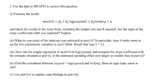
Gi) Estimate the model
math10 = fy + log(expend) + Bainchprg + u
‘and report the results in the usual form, including the sample size and R-squared. Are the signs of the
Slape coeficients what you expected? Explain.
(i) What do you make of the intercept you estimated in part )? In particular, does it make sense to
Set the two explanatory variables to zero? [Hint: Recal that og(1) = 0.)
il Now run the simple regression of math!) on logfexpend), and compare the slape coefficient with
the estimate obiained in part (i). s the estimated spending effet now larger or smaller than in part)?
(8) Find the corelation between lexpend = log(expend) and Inchprg. Docs its sign make sense to
you?
(4) Use part (iv) t0 explain your findings in parti).
Question:
Give step-by-step solution with explanation and final answer:2. Use the data in MEAPO3 to answer this question
Gi) Estimate the model
math10 = fy + log(expend) + Bainchprg + u
‘and report the results in the usual form, including the sample size and R-squared. Are the signs of the
Slape coeficients what you expected? Explain.
(i) What do you make of the intercept you estimated in part )? In particular, does it make sense to
Set the two explanatory variables to zero? [Hint: Recal that og(1) = 0.)
il Now run the simple regression of math!) on logfexpend), and compare the slape coefficient with
the estimate obiained in part (i). s the estimated spending effet now larger or smaller than in part)?
(8) Find the corelation between lexpend = log(expend) and Inchprg. Docs its sign make sense to
you?
(4) Use part (iv) t0 explain your findings in parti).
This is AI generated Response.
Asked by: Vikram Kumar
Created at: 2025-10-20 23:49:51
Final Answer:
RenderedRaw Text
Did you like this answer?
Let's go through each part step-by-step.
---
## Given Model
\[
\text{math10} = \beta_ + \beta_1 \log(\text{expend}) + \beta_2 \text{lnchprg} + u
\]
---
## (i) Estimate the model
**Note:** Since actual data is not provided, we'll explain the estimation process conceptually.
### Explanation:
- **Objective:** Find estimates for \(\beta_, \beta_1, \beta_2\).
- **Method:** Ordinary Least Squares (OLS).
- **Procedure:**
- Collect data on **expend**, **lnchprg**, and the dependent variable **math10**.
- Compute the logarithm of **expend** for each observation.
- Minimize the sum of squared residuals:
\[
\text{RSS} = \sum_{i=1}^n \left( \text{math10}_i - \beta_ - \beta_1 \log(\text{expend}_i) - \beta_2 \text{lnchprg}_i \right)^2
\]
- Solve the normal equations to estimate \(\hat{\beta}_, \hat{\beta}_1, \hat{\beta}_2\).
---
## (ii) Interpret the intercept (\(\beta_\))
- **Intercept (\(\beta_\))**: Estimated value of **math10** when \(\log(\text{expend})=\) and \(\text{lnchprg}=\).
- **Note:** \(\log(\text{expend})= \Rightarrow \text{expend}=1\), so the intercept is the expected **math10** score when **expend** is 1 unit and **lnchprg** is zero.
**Does it make sense to set the variables to zero?**
- For \(\text{lnchprg}=\), it depends on the context—possibly a baseline or minimal value.
- For \(\log(\text{expend})=\), **expend** equals 1, which might be a baseline.
---
## (iii) Run simple regression of **math10** on \(\log(\text{expend})\) only
\[
\text{math10} = \alpha_ + \alpha_1 \log(\text{expend}) + \epsilon
\]
### Compare slopes:
- **Estimate:** \(\hat{\alpha}_1\) from the simple regression.
- **Observation:** The slope in the multiple regression (\(\hat{\beta}_1\)) controls for the effect of **lnchprg**.
- **Expected outcome:**
- If **lnchprg** is correlated with **expend**, the slopes differ.
- Usually, **\(\hat{\beta}_1\)** (multiple regression) accounts for confounding and could be larger or smaller than \(\hat{\alpha}_1\).
**Question:** Is the slope larger or smaller in the multiple regression?
- It depends on the correlation between **lnchprg** and **expend** and their effect on **math10**.
---
## (iv) Correlation between **lnpend** and **expend**, and **lnchprg**
- **Correlation Significance:**
- If **lnpend** and **expend** are positively correlated, increases in expenditure associate with increases in **lnpend**.
- The sign of correlation affects multicollinearity and coefficient estimates.
- **Effect on regression:**
- High correlation may inflate standard errors.
- The sign of the correlation indicates whether the variables move together.
---
## (v) Use part (iv) to explain the change in slope coefficient
- If **lnpend** and **expend** are positively correlated:
- Omitting **lnpend** in the model could bias \(\beta_1\) upward if **lnpend** positively affects **math10**.
- Including **lnpend** controls for its effect, possibly reducing \(\beta_1\).
- The sign of the correlation informs whether the effect of **expend** is overestimated or underestimated when **lnpend** is omitted.
---
## Final notes:
- Precise numerical answers require actual data.
- The explanations above clarify the estimation, interpretation, and implications of correlations and regressions.
---
**Summary:**
- Estimation involves OLS with the transformed variables.
- The intercept is the expected **math10** score at baseline levels.
- Comparing simple and multiple regressions reveals how controlling for other variables affects the slope.
- Correlation impacts coefficient estimates and multicollinearity considerations.
Let me know if you'd like a simulated example or more detailed calculations!
VIPSolutions focuses on clear, step‑by‑step explanations so you can learn quickly. Whether you need an AI‑generated walkthrough or a short hint to get unstuck, each solution is organized for fast reading and easy review later.
Search similar questions, compare approaches, and bookmark the best answers for revision. Our goal is simple: quick, reliable study help that feels natural—not noisy.
 VIPSolutions
 2. Use the data in MEAPO3 to answer this question
Gi) Estimate the model
math10 = fy + log(expend) + Bainchprg + u
‘and report the results in the usual form, including the sample size and R-squared. Are the signs of the
Slape coeficients what you expected? Explain.
(i) What do you make of the intercept you estimated in part )? In particular, does it make sense to
Set the two explanatory variables to zero? [Hint: Recal that og(1) = 0.)
il Now run the simple regression of math!) on logfexpend), and compare the slape coefficient with
the estimate obiained in part (i). s the estimated spending effet now larger or smaller than in part)?
(8) Find the corelation between lexpend = log(expend) and Inchprg. Docs its sign make sense to
you?
(4) Use part (iv) t0 explain your findings in parti).