 VIPSolutions
Give step-by-step solution with explanation and final answer:You may submit your reports on the following questions: 1- The data in Table 7.6 show the survival times from diagnosis of patients suffering from leukemia. and the values of two explanatory variables, the white blood cell count (whe) and the presence or absence of a morpho- logical characteristic of the white blood cells (ag) (the data are available in package MASS, Venables and Ripley, 2002). 1. Define a binary outcome variable according to whether or not. patients lived for at least 24 weeks af- ter diagnosis. 2. Fit a logistic regression model to the data. It may be advisable to transform the very large white blood counts to avoid regression coefficients very close to 0 (and odds ratios very close to 1), and fit a model that contains only the two explanatory variables may not be adequate for these data. 3. Construct some graphics useful in the interpretation of the final model you fit. Table 7.6: Leuk data (package MASS). Survival times of patients suffering from lenkennis. Vor op time] whe we time TO preent G5 400 abeent 56 750 preent 156 | 3000 been 65 O00 preent 100 | 4000 abet 17 2000 present 134 | 1500 absent 7 600 preci 16| 0000 absn 16 10500 present 108 | 500 absent 2 10000 prescnt 121 | 1000 absent 3 TOD preent 4 | 1000 abe 4 S00 prea 30 | 2000 absent 2 TOO prescat 143 | 28000 absca 3 9400 preci 50 | 3000 abe 8 00 present 20| 20000 absent 4 3000 present 22| 20000 abet 3 100000 present 1| 000 absent 30 00000 present 1[ 100000 absent 4 000 present 5| 100000 absent 43 10000 present 65 2- This question should be answered using the Weekly data set, which is part of the ISLR package. This data is similar in nature to the Smarket data, except that it contains 1, 089 weekly returns for 21 years, from the beginning of 1990 to the end of 2010. 1. Produce some numerical and graphical summaries of the Weekly data. Do there appear to be any patterns? 2. Use the full data set to perform a logistic regression with Direction as the response and the five lag variables plus Volume as predictors. Use the summary function to print the results. Do any of the predictors appear to be statistically significant? If so, which ones? 3. Compute the confusion matrix. Explain what the confusion matrix is telling you about the types of mistakes made by logistic regression. 4. Now fit the logistic regression model using a training data period from 1990 to 2008, with Lag2 as the only predictor. Compute the confusion matrix and the overall fraction of correct predictions for the held out data (that is, the data from 2009 and 2010). 5. Repeat (part 4.) using LDA. 6. Repeat (part 4.) using QDA. 7. Which of these methods appears to provide the best results on this data?
Question:
Give step-by-step solution with explanation and final answer: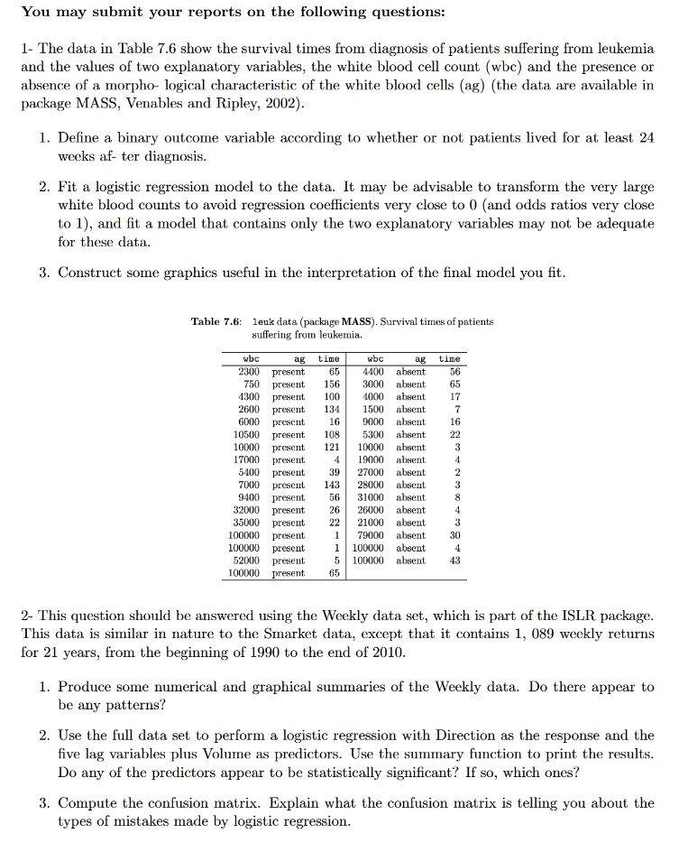
 You may submit your reports on the following questions:
1- The data in Table 7.6 show the survival times from diagnosis of patients suffering from leukemia.
and the values of two explanatory variables, the white blood cell count (whe) and the presence or
absence of a morpho- logical characteristic of the white blood cells (ag) (the data are available in
package MASS, Venables and Ripley, 2002).
1. Define a binary outcome variable according to whether or not. patients lived for at least 24
weeks af- ter diagnosis.
2. Fit a logistic regression model to the data. It may be advisable to transform the very large
white blood counts to avoid regression coefficients very close to 0 (and odds ratios very close
to 1), and fit a model that contains only the two explanatory variables may not be adequate
for these data.
3. Construct some graphics useful in the interpretation of the final model you fit.
Table 7.6: Leuk data (package MASS). Survival times of patients
suffering from lenkennis.
Vor op time] whe we time
TO preent G5 400 abeent 56
750 preent 156 | 3000 been 65
O00 preent 100 | 4000 abet 17
2000 present 134 | 1500 absent 7
600 preci 16| 0000 absn 16
10500 present 108 | 500 absent 2
10000 prescnt 121 | 1000 absent 3
TOD preent 4 | 1000 abe 4
S00 prea 30 | 2000 absent 2
TOO prescat 143 | 28000 absca 3
9400 preci 50 | 3000 abe 8
00 present 20| 20000 absent 4
3000 present 22| 20000 abet 3
100000 present 1| 000 absent 30
00000 present 1[ 100000 absent 4
000 present 5| 100000 absent 43
10000 present 65
2- This question should be answered using the Weekly data set, which is part of the ISLR package.
This data is similar in nature to the Smarket data, except that it contains 1, 089 weekly returns
for 21 years, from the beginning of 1990 to the end of 2010.
1. Produce some numerical and graphical summaries of the Weekly data. Do there appear to
be any patterns?
2. Use the full data set to perform a logistic regression with Direction as the response and the
five lag variables plus Volume as predictors. Use the summary function to print the results.
Do any of the predictors appear to be statistically significant? If so, which ones?
3. Compute the confusion matrix. Explain what the confusion matrix is telling you about the
types of mistakes made by logistic regression.
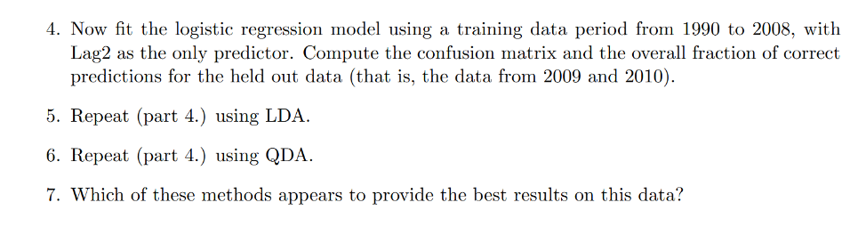
4. Now fit the logistic regression model using a training data period from 1990 to 2008, with
Lag2 as the only predictor. Compute the confusion matrix and the overall fraction of correct
predictions for the held out data (that is, the data from 2009 and 2010).
5. Repeat (part 4.) using LDA.
6. Repeat (part 4.) using QDA.
7. Which of these methods appears to provide the best results on this data?
Asked by: venky
Created at: 2025-09-27 07:40:56
Final Answer:
📢 Instructions:
- Ask anything relatd to above question only.
- For new Question goto :