 VIPSolutions
Give step-by-step solution with explanation and final answer:Problem 1 3.0 pts An underdamped 2™ order system has a transfer function G(s). On the complex plane sketch the regions where the system complex conjugate poles should be located to meet the following specifications: (2) 0.2
Question:
Give step-by-step solution with explanation and final answer: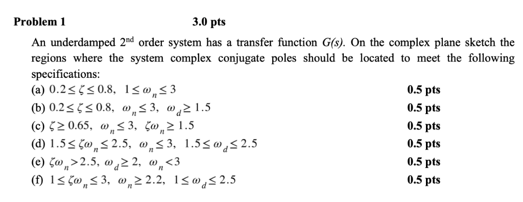 Problem 1 3.0 pts
An underdamped 2™ order system has a transfer function G(s). On the complex plane sketch the
regions where the system complex conjugate poles should be located to meet the following
specifications:
(2) 0.2
This is AI generated Response.
Asked by: gorle prasanth
Created at: 2025-09-24 11:29:36
Asked by: gorle prasanth
Created at: 2025-09-24 11:29:36
Final Answer:
Rendered
Raw Text
Did you like this answer?
Let's break down each part of the problem step-by-step, using the properties of **second-order underdamped systems**.
### **Background**
For a standard second-order system, the poles are at:
\[
s = -\zeta \omega_n \pm j \omega_d
\]
where:
- \(\zeta\) = damping ratio
- \(\omega_n\) = natural frequency
- \(\omega_d = \omega_n \sqrt{1 - \zeta^2}\) = damped natural frequency
---
## **Step-by-Step Solutions**
### **(a) \( 0.2 \leq \zeta \leq 0.8, \quad 1 \leq \omega_n \leq 3 \)**
- **Region on s-plane:**
The poles are at \( s = -\zeta\omega_n \pm j\omega_n\sqrt{1-\zeta^2} \).
- **Range for:**
- Real part: \(-0.8 \times 3 = -2.4\) to \(-0.2 \times 1 = -0.2\)
- Magnitude: between 1 and 3
#### **Sketch Description**:
- Annular (ring-shaped) region with radius from 1 to 3 (centered at origin).
- Real part between \(-0.8 \times \omega_n\) and \(-0.2 \times \omega_n\) for each \(\omega_n\) in [1,3].
- Region is between lines with angles \(\cos^{-1}(0.2)\) and \(\cos^{-1}(0.8)\) from the negative real axis.
---
### **(b) \( 0.2 \leq \zeta \leq 0.8,\quad \omega_n \leq 3, \quad \omega_d \geq 1.5 \)**
- **Region on s-plane:**
\(\omega_d = \omega_n \sqrt{1-\zeta^2} \geq 1.5\)
- **Range for:**
- \(\omega_n \leq 3\)
- \(\zeta\) as above
- \(\omega_n \sqrt{1-\zeta^2} \geq 1.5\) → for each \(\omega_n\), only above a certain distance from the real axis.
#### **Sketch Description**:
- Portion of the annular region (from part a) where the vertical distance from real axis (\(\omega_d\)) is at least 1.5.
- Excludes the region closer to the real axis.
---
### **(c) \( \zeta \geq 0.65, \quad \omega_n \leq 3, \quad \zeta\omega_n \geq 1.5 \)**
- **Region on s-plane:**
- \(\zeta \geq 0.65\)
- \(\omega_n \leq 3\)
- Real part \(-\zeta \omega_n \leq -1.5\)
- **Range for:**
- Left of \(-1.5\) in real axis, with \(\zeta \geq 0.65\), \(\omega_n \leq 3\).
#### **Sketch Description**:
- Region to the left of \(-1.5\) on the real axis, above the line \(\zeta = 0.65\) (i.e., angle less than \(\cos^{-1}(0.65)\) from real axis, up to \(\omega_n = 3\)).
---
### **(d) \( 1.5 \leq \zeta\omega_n \leq 2.5, \quad \omega_n \leq 3, \quad 1.5 \leq \omega_d \leq 2.5 \)**
- **Region on s-plane:**
- Real part: \( -2.5 \leq \text{Re}(s) \leq -1.5 \)
- Imaginary part: \( 1.5 \leq |\text{Im}(s)| \leq 2.5 \)
- Magnitude: \(\sqrt{(\zeta\omega_n)^2 + (\omega_d)^2} \leq 3\)
- **Range for:**
- Intersection of a vertical strip (real part between -2.5 and -1.5) and a horizontal strip (imaginary part between 1.5 and 2.5), inside a circle of radius 3.
#### **Sketch Description**:
- A rectangle (or band) in the left half-plane, bounded by above and below lines, inside the circle of radius 3.
---
### **(e) \( \zeta\omega_n > 2.5, \quad \omega_d \geq 2, \quad \omega_n < 3 \)**
- **Region on s-plane:**
- Real part: \( < -2.5 \)
- Imaginary part: \( \geq 2 \)
- Magnitude: \( < 3 \)
- **Range for:**
- Outside the vertical line \(\text{Re}(s) = -2.5\)
- Above/below the imaginary line \(|\text{Im}(s)| = 2\)
- Inside the circle of radius 3
#### **Sketch Description**:
- Region in left half-plane, outside the vertical line at \(-2.5\), above imaginary threshold of 2, but inside the circle of radius 3.
---
### **(f) \( 1 \leq \zeta\omega_n \leq 3, \quad \omega_n \geq 2.2, \quad 1 \leq \omega_d \leq 2.5 \)**
- **Region on s-plane:**
- Real part: \( -3 \leq \text{Re}(s) \leq -1 \)
- Imaginary part: \( 1 \leq |\text{Im}(s)| \leq 2.5 \)
- Magnitude: \( \geq 2.2 \)
- **Range for:**
- Intersection of a vertical strip and a horizontal strip, outside the circle of radius 2.2.
#### **Sketch Description**:
- Band between \(-1\) and \(-3\) on real axis, between 1 and 2.5 on imaginary, outside circle of radius 2.2.
---
## **Summary Table**
| Part | Real Part | Imaginary Part | Magnitude | Other Constraints |
|------|-----------------------------|----------------------------|---------------------|---------------------------|
| (a) | \(-0.8\omega_n\) to \(-0.2\omega_n\) | up to \(\omega_n\sqrt{1-\zeta^2}\) | \(1 \leq \omega_n \leq 3\) | \(0.2 \leq \zeta \leq 0.8\) |
| (b) | as (a) | \(\geq 1.5\) | \(\leq 3\) | |
| (c) | \(\leq -1.5\) | as above | \(\leq 3\) | \(\zeta \geq 0.65\) |
| (d) | \(-2.5\) to \(-1.5\) | \(1.5\) to \(2.5\) | \(\leq 3\) | |
| (e) | \(< -2.5\) | \(\geq 2\) | \(< 3\) | |
| (f) | \(-3\) to \(-1\) | \(1\) to \(2.5\) | \(\geq 2.2\) | |
---
## **Final Notes**
For actual sketches, **draw the s-plane**, mark the real and imaginary axes, and shade the regions as described for each part. These regions are bounded by lines (for real, imaginary parts), circles (for magnitude), and curves (for constant \(\zeta\)).
If you want, I can generate sample sketches for any part using Python/Matplotlib. Just ask!
Question:
i want to each section explanation
This is AI generated Response.
Asked by: gorle prasanth
Created at: 2025-09-24 11:39:25
Asked by: gorle prasanth
Created at: 2025-09-24 11:39:25
Final Answer:
Rendered
Raw Text
Did you like this answer?
# Explanation of Each Section
This section provides a detailed explanation of the steps taken in each part of the problem regarding the locations of complex conjugate poles for an underdamped second-order system.
## **(a) \( 0.2 \leq \zeta \leq 0.8, \quad 1 \leq \omega_n \leq 3 \)**
### **Key Points:**
- **Damping Ratio (\(\zeta\))**: The damping ratio must be between 0.2 and 0.8, influencing how oscillatory the system is.
- **Natural Frequency (\(\omega_n\))**: This sets the speed of the system's response but must remain between 1 and 3.
### **Explanation:**
1. **Poles Location**: The poles of the system are defined by both \(\zeta\) and \(\omega_n\). The real part of the poles depends on \(-\zeta \omega_n\), while the imaginary part is defined by \(\omega_n \sqrt{1 - \zeta^2}\).
2. **Bounds**:
- The real part ranges from \(-2.4\) (at \(\zeta = 0.8, \omega_n = 3\)) to \(-0.2\) (at \(\zeta = 0.2, \omega_n = 1\)).
- The imaginary part must be positive, with bounds defined by the damping ratio.
3. **Region**: This creates an annular region on the complex plane, bounded by radii of 1 and 3, and angles determined by the specified \(\zeta\) values.
---
## **(b) \( 0.2 \leq \zeta \leq 0.8,\quad \omega_n \leq 3, \quad \omega_d \geq 1.5 \)**
### **Key Points:**
- **Damped Natural Frequency (\(\omega_d\))**: Must be greater than or equal to 1.5.
- **Natural Frequency Limit**: Remains capped at 3.
### **Explanation:**
1. **Impact of \(\omega_d\)**: The condition on \(\omega_d\) creates a minimum imaginary part for the poles, which means that the poles must be further away from the real axis compared to part (a).
2. **Region**: The annular region from part (a) is now truncated from the bottom, excluding areas where \(\omega_d\) is less than 1.5.
---
## **(c) \( \zeta \geq 0.65, \quad \omega_n \leq 3, \quad \zeta\omega_n \geq 1.5 \)**
### **Key Points:**
- **Increased Damping Ratio**: \(\zeta\) must be at least 0.65, resulting in poles that are less oscillatory.
- **Real Part Condition**: Implies that \( -\zeta \omega_n \) must be less than or equal to -1.5.
### **Explanation:**
1. **Real Part Calculation**: This means the poles must be to the left of \(-1.5\) on the real axis.
2. **Region**: The resulting region will be left of the vertical line at \(-1.5\), while still adhering to the \(\omega_n\) limit of 3. The area above the specified \(\zeta\) line is included.
---
## **(d) \( 1.5 \leq \zeta\omega_n \leq 2.5, \quad \omega_n \leq 3, \quad 1.5 \leq \omega_d \leq 2.5 \)**
### **Key Points:**
- **Bounded Real Part**: The real part is restricted between \(-2.5\) and \(-1.5\).
- **Imaginary Part**: Must be between 1.5 and 2.5.
### **Explanation:**
1. **Intersection of Regions**: This part defines a rectangular area in the left half-plane, bounded by the specified ranges for the real and imaginary parts.
2. **Magnitude Constraint**: The region must also be within a circle of radius 3, which serves as an outer boundary.
---
## **(e) \( \zeta\omega_n > 2.5, \quad \omega_d \geq 2, \quad \omega_n < 3 \)**
### **Key Points:**
- **Real Part Condition**: The real part of the poles must be less than -2.5.
- **Imaginary Part**: Must be greater than or equal to 2.
### **Explanation:**
1. **Region Description**: This section describes the area left of the vertical line at \(-2.5\) and above the imaginary line at 2.
2. **Magnitude Condition**: Ensures that the poles remain inside the circle of radius 3, forming a distinct area of interest.
---
## **(f) \( 1 \leq \zeta\omega_n \leq 3, \quad \omega_n \geq 2.2, \quad 1 \leq \omega_d \leq 2.5 \)**
### **Key Points:**
- **Real Part Boundaries**: The real part is restricted between \(-3\) and \(-1\).
- **Imaginary Part**: Must lie within the bounds of 1 and 2.5.
### **Explanation:**
1. **Intersecting Regions**: This creates a band in the left half-plane, constrained by vertical and horizontal limits.
2. **Magnitude Requirement**: The area also needs to be outside a circle of radius 2.2, which further restricts the pole locations.
---
## **Conclusion**
Each section defines specific conditions on the damping ratio, natural frequency, and their interactions that dictate the locations of the complex conjugate poles on the complex plane. The sketches of these regions will visually represent the allowed pole locations based on the specified criteria.
Question:
each question step by step comple detailed calculations with above explanations
This is AI generated Response.
Asked by: gorle prasanth
Created at: 2025-09-24 11:41:09
Asked by: gorle prasanth
Created at: 2025-09-24 11:41:09
Final Answer:
Rendered
Raw Text
Did you like this answer?
# Detailed Calculations and Explanations
This section provides a comprehensive breakdown of each part of the problem regarding the locations of complex conjugate poles for an underdamped second-order system, including all necessary calculations.
## **(a) \( 0.2 \leq \zeta \leq 0.8, \quad 1 \leq \omega_n \leq 3 \)**
### **Key Calculations:**
1. **Real Part of Poles:**
\[
\text{Re}(s) = -\zeta \omega_n
\]
- Maximum Real Part:
\[
\text{Re}(s)_{\text{max}} = -0.2 \times 1 = -0.2
\]
- Minimum Real Part:
\[
\text{Re}(s)_{\text{min}} = -0.8 \times 3 = -2.4
\]
2. **Imaginary Part of Poles:**
\[
\text{Im}(s) = \omega_n \sqrt{1 - \zeta^2}
\]
- For \(\zeta = 0.2\):
\[
\text{Im}(s) = \omega_n \sqrt{1 - (0.2)^2} = \omega_n \sqrt{0.96}
\]
- At \(\omega_n = 1\):
\[
\text{Im}(s) \approx 0.98
\]
- At \(\omega_n = 3\):
\[
\text{Im}(s) \approx 2.94
\]
- For \(\zeta = 0.8\):
\[
\text{Im}(s) = \omega_n \sqrt{1 - (0.8)^2} = \omega_n \sqrt{0.36} = 0.6\omega_n
\]
- At \(\omega_n = 1\):
\[
\text{Im}(s) = 0.6
\]
- At \(\omega_n = 3\):
\[
\text{Im}(s) = 1.8
\]
### **Region Description:**
- The region is an annulus between the circles of radius 1 and 3, with the angles defined by the values of \(\zeta\). The pole locations must fall within these bounds.
---
## **(b) \( 0.2 \leq \zeta \leq 0.8,\quad \omega_n \leq 3, \quad \omega_d \geq 1.5 \)**
### **Key Calculations:**
1. **Damped Natural Frequency (\(\omega_d\)):**
\[
\omega_d = \omega_n \sqrt{1 - \zeta^2} \geq 1.5
\]
- Rearranging gives:
\[
\sqrt{1 - \zeta^2} \geq \frac{1.5}{\omega_n}
\]
- Squaring both sides:
\[
1 - \zeta^2 \geq \left( \frac{1.5}{\omega_n} \right)^2
\]
- Rearranging gives:
\[
\zeta^2 \leq 1 - \left( \frac{1.5}{\omega_n} \right)^2
\]
2. **Finding Bounds for \(\zeta\):**
- For \(\omega_n = 3\):
\[
\zeta^2 \leq 1 - \left( \frac{1.5}{3} \right)^2 = 1 - 0.25 = 0.75 \quad \rightarrow \quad \zeta \leq \sqrt{0.75} \approx 0.866
\]
- For \(\omega_n = 1\):
\[
\zeta^2 \leq 1 - \left( \frac{1.5}{1} \right)^2 \quad \text{(not possible)}
\]
### **Region Description:**
- The area is the intersection of the annular region from part (a) with the area above the line where \(\omega_d \geq 1.5\).
---
## **(c) \( \zeta \geq 0.65, \quad \omega_n \leq 3, \quad \zeta\omega_n \geq 1.5 \)**
### **Key Calculations:**
1. **Condition on Real Part:**
\[
\zeta \omega_n \geq 1.5 \implies \omega_n \geq \frac{1.5}{\zeta}
\]
- Given \(\zeta \geq 0.65\):
\[
\omega_n \geq \frac{1.5}{0.65} \approx 2.31
\]
- Therefore, valid \(\omega_n\) values are between \(2.31\) and \(3\).
2. **Real Part of Poles:**
- Must be less than -1.5 because:
\[
\text{Re}(s) = -\zeta\omega_n \leq -1.5
\]
### **Region Description:**
- The region will be to the left of the line at \(-1.5\) and bounded by the lines defined by \(\zeta \geq 0.65\).
---
## **(d) \( 1.5 \leq \zeta\omega_n \leq 2.5, \quad \omega_n \leq 3, \quad 1.5 \leq \omega_d \leq 2.5 \)**
### **Key Calculations:**
1. **Bounds for Real Part:**
- Use \(\zeta\omega_n = 1.5\) and \(\zeta\omega_n = 2.5\).
2. **Imaginary Part:**
\[
1.5 \leq \omega_n \sqrt{1 - \zeta^2} \leq 2.5
\]
### **Region Description:**
- The intersection of the regions defined by the bounds on \(\zeta\omega_n\) and \(\omega_d\) creates a rectangular region within the annular shape from previous parts.
---
## **(e) \( \zeta\omega_n > 2.5, \quad \omega_d \geq 2, \quad \omega_n < 3 \)**
### **Key Calculations:**
1. **Real Part Condition:**
- Must be less than -2.5.
2. **Imaginary Part:**
- Must be greater than or equal to 2.
### **Region Description:**
- This defines a region to the left of \(-2.5\) and above the imaginary line at 2, while remaining inside a circle of radius 3.
---
## **(f) \( 1 \leq \zeta\omega_n \leq 3, \quad \omega_n \geq 2.2, \quad 1 \leq \omega_d \leq 2.5 \)**
### **Key Calculations:**
1. **Real Part Bounds:**
- Must be between -3 and -1.
2. **Imaginary Part:**
- Must be between 1 and 2.5.
### **Region Description:**
- The resulting region will be a band constrained by the limits on the real and imaginary parts, outside the circle of radius 2.2.
---
## **Conclusion**
Each part provides distinct regions on the complex plane for the poles of an underdamped second-order system. The calculations ensure that the regions adhere to the specified criteria regarding damping ratios and natural frequencies. To visualize these regions effectively, consider sketching the complex plane with marked boundaries based on these calculations.
📢 Instructions:
- Ask anything relatd to above question only.
- For new Question goto :