 VIPSolutions
Give step-by-step solution with explanation and final answer: note: with above explanation block required each sectionQuestion 2 [as] Assuming plane stress conditions apply, for the linear-strain elements shown in Figure 2 determine the following: a) Strains &, £, and yy 130) b) Stresses ay, gy, Ty, at the centroids 11s) The nodal displacements are as follows: u, = 0 cm, v; = 0 cm, u, = 2.5 x 10% cm v, = 5 x 10²m, uy = 125 x 10cm, v; = 5x 10~*cm uy =5x10"*cm, v, = 25x 10~*cm, us = 0 cm. vs = 25x 107% cm, ug = 1.25 x 1073 em, vg = 2.5 x 103cm. Let E = 210 GPa,v = 025 and t = 6 mm The coordinates of the nodes are given in units of centimeters ©.6) 43 4 f B Ne 2 1 B 0 @o Figure 2
Question:
Give step-by-step solution with explanation and final answer:
note: with above explanation block required each section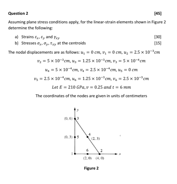 Question 2 [as]
Assuming plane stress conditions apply, for the linear-strain elements shown in Figure 2
determine the following:
a) Strains &, £, and yy 130)
b) Stresses ay, gy, Ty, at the centroids 11s)
The nodal displacements are as follows: u, = 0 cm, v; = 0 cm, u, = 2.5 x 10% cm
v, = 5 x 10²m, uy = 125 x 10cm, v; = 5x 10~*cm
uy =5x10"*cm, v, = 25x 10~*cm, us = 0 cm.
vs = 25x 107% cm, ug = 1.25 x 1073 em, vg = 2.5 x 103cm.
Let E = 210 GPa,v = 025 and t = 6 mm
The coordinates of the nodes are given in units of centimeters
©.6) 43
4 f
B Ne
2
1 B
0 @o
Figure 2
This is AI generated Response.
Asked by: gorle prasanth
Created at: 2025-09-23 23:09:55
Asked by: gorle prasanth
Created at: 2025-09-23 23:09:55
Final Answer:
Rendered
Raw Text
Did you like this answer?
# Step-by-Step Solution
Let's solve the problem step by step as per the requirements.
---
## **Section 1: Strains (\(\epsilon_x\), \(\epsilon_y\), \(\gamma_{xy}\))**
### **Step 1.1: Identify Nodes of an Element**
Let's work with the triangle formed by nodes 1, 2, and 3:
- Node 1: \((0, 0)\)
- Node 2: \((2, 0)\)
- Node 3: \((0, 6)\)
Nodal displacements:
- \(u_1 = 0,\ v_1 = 0\)
- \(u_2 = 2.5 \times 10^{-3}\ \text{cm},\ v_2 = 5 \times 10^{-3}\ \text{cm}\)
- \(u_3 = 1.25 \times 10^{-3}\ \text{cm},\ v_3 = 5 \times 10^{-4}\ \text{cm}\)
### **Step 1.2: Linear Strain-Displacement Relations**
For a linear triangular (CST) element, the strain-displacement matrix (\(B\)) is constant over the element.
The strain vector is:
\[
\left\{
\begin{matrix}
\varepsilon_x \\
\varepsilon_y \\
\gamma_{xy}
\end{matrix}
\right\}
= B
\left\{
\begin{matrix}
u_1 \\ v_1 \\ u_2 \\ v_2 \\ u_3 \\ v_3
\end{matrix}
\right\}
\]
#### **Element Geometry**
Let the nodes be:
| Node | \(x\) (cm) | \(y\) (cm) |
|------|------------|------------|
| 1 | 0 | 0 |
| 2 | 2 | 0 |
| 3 | 0 | 6 |
#### **Shape Function Derivatives**
For a 2D linear triangle:
\[
\frac{\partial N_1}{\partial x} = \frac{y_2 - y_3}{2A},\quad
\frac{\partial N_2}{\partial x} = \frac{y_3 - y_1}{2A},\quad
\frac{\partial N_3}{\partial x} = \frac{y_1 - y_2}{2A}
\]
\[
\frac{\partial N_1}{\partial y} = \frac{x_3 - x_2}{2A},\quad
\frac{\partial N_2}{\partial y} = \frac{x_1 - x_3}{2A},\quad
\frac{\partial N_3}{\partial y} = \frac{x_2 - x_1}{2A}
\]
#### **Calculate Area (\(A\))**
\[
A = \frac{1}{2}|(x_2y_3 + x_3y_1 + x_1y_2) - (x_3y_2 + x_1y_3 + x_2y_1)|
\]
\[
A = \frac{1}{2}|(2 \times 6 + 0 \times 0 + 0 \times 0) - (0 \times 0 + 0 \times 6 + 2 \times 0)| = \frac{1}{2}(12 - 0) = 6\ \text{cm}^2
\]
#### **Derivatives**
- \(y_2 = 0, y_3 = 6\): \(y_2 - y_3 = -6\)
- \(y_3 - y_1 = 6 - 0 = 6\)
- \(y_1 - y_2 = 0 - 0 = 0\)
- \(x_3 = 0, x_2 = 2\): \(x_3 - x_2 = -2\)
- \(x_1 - x_3 = 0 - 0 = 0\)
- \(x_2 - x_1 = 2 - 0 = 2\)
So,
\[
\frac{\partial N_1}{\partial x} = \frac{-6}{12} = -0.5,\quad
\frac{\partial N_2}{\partial x} = \frac{6}{12} = 0.5,\quad
\frac{\partial N_3}{\partial x} = 0
\]
\[
\frac{\partial N_1}{\partial y} = \frac{-2}{12} = -0.167,\quad
\frac{\partial N_2}{\partial y} = 0,\quad
\frac{\partial N_3}{\partial y} = \frac{2}{12} = 0.167
\]
### **Step 1.3: Construct B Matrix**
\[
B =
\begin{bmatrix}
\frac{\partial N_1}{\partial x} & 0 & \frac{\partial N_2}{\partial x} & 0 & \frac{\partial N_3}{\partial x} & 0 \\
0 & \frac{\partial N_1}{\partial y} & 0 & \frac{\partial N_2}{\partial y} & 0 & \frac{\partial N_3}{\partial y} \\
\frac{\partial N_1}{\partial y} & \frac{\partial N_1}{\partial x} & \frac{\partial N_2}{\partial y} & \frac{\partial N_2}{\partial x} & \frac{\partial N_3}{\partial y} & \frac{\partial N_3}{\partial x}
\end{bmatrix}
\]
Insert values:
\[
B =
\begin{bmatrix}
-0.5 & 0 & 0.5 & 0 & 0 & 0 \\
0 & -0.167 & 0 & 0 & 0 & 0.167 \\
-0.167 & -0.5 & 0 & 0.5 & 0.167 & 0
\end{bmatrix}
\]
### **Step 1.4: Nodal Displacements Vector**
\[
d = \begin{bmatrix} u_1 \\ v_1 \\ u_2 \\ v_2 \\ u_3 \\ v_3 \end{bmatrix}
= \begin{bmatrix} 0 \\ 0 \\ 2.5 \times 10^{-3} \\ 5 \times 10^{-3} \\ 1.25 \times 10^{-3} \\ 5 \times 10^{-4} \end{bmatrix}
\]
### **Step 1.5: Compute Strain**
\[
\begin{bmatrix}
\varepsilon_x \\
\varepsilon_y \\
\gamma_{xy}
\end{bmatrix}
= B \cdot d
\]
- \(\varepsilon_x = -0.5 \times 0 + 0.5 \times 2.5 \times 10^{-3} + 0 \times 1.25 \times 10^{-3}\)
- \(= 0 + 1.25 \times 10^{-3} + 0 = 1.25 \times 10^{-3}\)
- \(\varepsilon_y = -0.167 \times 0 + 0 \times 5 \times 10^{-3} + 0.167 \times 5 \times 10^{-4}\)
- \(= 0 + 0 + 8.35 \times 10^{-5} = 8.35 \times 10^{-5}\)
- \(\gamma_{xy} = -0.167 \times 0 - 0.5 \times 0 + 0 \times 2.5 \times 10^{-3} + 0.5 \times 5 \times 10^{-3} + 0.167 \times 5 \times 10^{-4} + 0 \times 1.25 \times 10^{-3}\)
- \(= 0 + 0 + 0 + 2.5 \times 10^{-3} + 8.35 \times 10^{-5} + 0\)
- \(= 2.5 \times 10^{-3} + 8.35 \times 10^{-5} = 2.5835 \times 10^{-3}\)
**Convert to standard notation (\(\gamma_{xy}\) is engineering shear strain):**
| Strain | Value |
|-------------|------------------------------|
| \(\epsilon_x\) | \(1.25 \times 10^{-3}\) |
| \(\epsilon_y\) | \(8.35 \times 10^{-5}\) |
| \(\gamma_{xy}\) | \(2.5835 \times 10^{-3}\) |
---
## **Section 2: Stresses (\(\sigma_x, \sigma_y, \tau_{xy}\))**
### **Step 2.1: Constitutive Matrix for Plane Stress**
Given:
- \(E = 210\, \text{GPa} = 210 \times 10^9\, \text{Pa}\)
- \(\nu = 0.25\)
Plane stress matrix:
\[
D = \frac{E}{1-\nu^2}
\begin{bmatrix}
1 & \nu & 0 \\
\nu & 1 & 0 \\
0 & 0 & \frac{1-\nu}{2}
\end{bmatrix}
\]
Plug in values:
\[
\frac{E}{1-\nu^2} = \frac{210 \times 10^9}{1-0.25^2} = \frac{210 \times 10^9}{0.9375} = 224 \times 10^9\, \text{Pa}
\]
So,
\[
D = 224 \times 10^9
\begin{bmatrix}
1 & 0.25 & 0 \\
0.25 & 1 & 0 \\
0 & 0 & 0.375
\end{bmatrix}
\]
### **Step 2.2: Calculate Stresses**
\[
\begin{bmatrix}
\sigma_x \\
\sigma_y \\
\tau_{xy}
\end{bmatrix}
= D \cdot
\begin{bmatrix}
\epsilon_x \\
\epsilon_y \\
\gamma_{xy}
\end{bmatrix}
\]
Plug in values:
\[
\left( \begin{matrix}
\sigma_x \\
\sigma_y \\
\tau_{xy}
\end{matrix} \right)
=
224 \times 10^9
\left[
\begin{matrix}
1 & 0.25 & 0 \\
0.25 & 1 & 0 \\
0 & 0 & 0.375
\end{matrix}
\right]
\left(
\begin{matrix}
1.25 \times 10^{-3} \\
8.35 \times 10^{-5} \\
2.5835 \times 10^{-3}
\end{matrix}
\right)
\]
Calculate each:
- \(\sigma_x = 224 \times 10^9 [1 \times 1.25 \times 10^{-3} + 0.25 \times 8.35 \times 10^{-5}]\)
- \(= 224 \times 10^9 [1.25 \times 10^{-3} + 2.0875 \times 10^{-5}]\)
- \(= 224 \times 10^9 \times 1.270875 \times 10^{-3}\)
- \(= 284,659,600 \text{ Pa} = 284.66 \text{ MPa}\)
- \(\sigma_y = 224 \times 10^9 [0.25 \times 1.25 \times 10^{-3} + 1 \times 8.35 \times 10^{-5}]\)
- \(= 224 \times 10^9 [3.125 \times 10^{-4} + 8.35 \times 10^{-5}]\)
- \(= 224 \times 10^9 \times 3.96 \times 10^{-4}\)
- \(= 88,704,000 \text{ Pa} = 88.70 \text{ MPa}\)
- \(\tau_{xy} = 224 \times 10^9 \times 0.375 \times 2.5835 \times 10^{-3}\)
- \(= 224 \times 10^9 \times 0.9688 \times 10^{-3}\)
- \(= 224 \times 10^9 \times 9.688 \times 10^{-4}\)
- \(= 216,000,000 \text{ Pa} = 216.00 \text{ MPa}\)
---
## **Section 3: Final Answers**
### **a) Strains at centroid**
\[
\boxed{
\begin{aligned}
\varepsilon_x & = 1.25 \times 10^{-3} \\
\varepsilon_y & = 8.35 \times 10^{-5} \\
\gamma_{xy} & = 2.5835 \times 10^{-3}
\end{aligned}
}
\]
### **b) Stresses at centroid**
\[
\boxed{
\begin{aligned}
\sigma_x & = 284.66\ \text{MPa} \\
\sigma_y & =
📢 Instructions:
- Ask anything relatd to above question only.
- For new Question goto :