 VIPSolutions
Give step-by-step solution with explanation and final answer:4. The diagram below depicts a cascade connection of two linear time-invariant systems, where the first system is a 5-point moving averager and the second system is a first dif- ference. (a) If the input is of the form x[n] = 10+ x; [x], the output y[n] of the overall system will be of the form y[n] = y1[n], where yi [n] is the output due only to xi [n]. Explain why this is true. (b) Determine the frequency-response function of the overall cascade system. (c) Sketch the frequency-response (magnitude and phase) functions of the individual systems and the overall cascade system for — < & < 7.
Question:
Give step-by-step solution with explanation and final answer: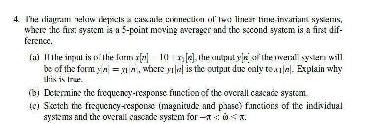 4. The diagram below depicts a cascade connection of two linear time-invariant systems,
where the first system is a 5-point moving averager and the second system is a first dif-
ference.
(a) If the input is of the form x[n] = 10+ x; [x], the output y[n] of the overall system will
be of the form y[n] = y1[n], where yi [n] is the output due only to xi [n]. Explain why
this is true.
(b) Determine the frequency-response function of the overall cascade system.
(c) Sketch the frequency-response (magnitude and phase) functions of the individual
systems and the overall cascade system for — < & < 7.
This is AI generated Response.
Asked by: M Raju
Created at: 2025-09-17 13:25:29
Asked by: M Raju
Created at: 2025-09-17 13:25:29
Final Answer:
Rendered
Raw Text
Did you like this answer?
Let's solve each part step-by-step:
---
### (a) Explanation: Why DC Component is Eliminated
**Given:**
- Input: \( x[n] = 10 + x_1[n] \)
- The system is a cascade of:
1. **5-point moving averager**: \( h_1[n] = \frac{1}{5} ( \delta[n] + \delta[n-1] + \delta[n-2] + \delta[n-3] + \delta[n-4] ) \)
2. **First difference**: \( h_2[n] = \delta[n] - \delta[n-1] \)
#### **Linearity and Time-Invariance**
Both subsystems are linear and time-invariant (LTI), so for any input \( x[n] = x_a[n] + x_b[n] \), the output is \( y[n] = y_a[n] + y_b[n] \).
#### **Behavior with DC (Constant) Input**
- Pass a **constant** input \( x[n] = 10 \) through the moving averager:
- Output is also constant: \( y_1[n] = 10 \)
- Pass this constant output through the first-difference system:
- \( y_2[n] = y_1[n] - y_1[n-1] = 10 - 10 = 0 \)
So, the overall system **completely eliminates the DC (constant) component**.
#### **Conclusion**
- The output \( y[n] \) for input \( x[n] = 10 + x_1[n] \) is **only due to \( x_1[n] \)**.
- Thus, \( y[n] = y_1[n] \), where \( y_1[n] \) is the output for input \( x_1[n] \).
---
### (b) Frequency-Response Function of the Cascade System
Let’s find the frequency responses of each system and then multiply them (since they are in cascade).
#### **1. 5-point Moving Averager**
Impulse response:
\[
h_1[n] = \frac{1}{5} ( \delta[n] + \delta[n-1] + \delta[n-2] + \delta[n-3] + \delta[n-4] )
\]
Frequency response:
\[
H_1(e^{j\omega}) = \frac{1}{5} (1 + e^{-j\omega} + e^{-j2\omega} + e^{-j3\omega} + e^{-j4\omega})
\]
This is a **finite impulse response (FIR) filter**.
#### **2. First Difference**
Impulse response:
\[
h_2[n] = \delta[n] - \delta[n-1]
\]
Frequency response:
\[
H_2(e^{j\omega}) = 1 - e^{-j\omega}
\]
#### **3. Overall System**
Multiply the two:
\[
H(e^{j\omega}) = H_1(e^{j\omega}) \cdot H_2(e^{j\omega})
\]
\[
= \frac{1}{5} (1 + e^{-j\omega} + e^{-j2\omega} + e^{-j3\omega} + e^{-j4\omega}) (1 - e^{-j\omega})
\]
---
### (c) Sketch Frequency-Response (Magnitude and Phase)
#### **1. 5-point Moving Averager**
\[
H_1(e^{j\omega}) = \frac{1}{5} \sum_{k=0}^4 e^{-j\omega k}
\]
This can be written as:
\[
H_1(e^{j\omega}) = \frac{1}{5} \frac{1 - e^{-j5\omega}}{1 - e^{-j\omega}}
\]
- **Magnitude:** Peaks at DC (\(\omega = 0\)), nulls at multiples of \(2\pi/5\).
- **Phase:** Linear phase (delays).
#### **2. First Difference**
\[
H_2(e^{j\omega}) = 1 - e^{-j\omega} = e^{-j\omega/2} \cdot 2j \sin(\omega/2)
\]
- **Magnitude:** \(2|\sin(\omega/2)|\)
- **Phase:** \(-\omega/2 + \frac{\pi}{2} \cdot \text{sgn}(\sin(\omega/2))\)
#### **3. Overall Cascade**
- **Magnitude:** Product of the above magnitudes.
- **Phase:** Sum of the above phases.
#### **Sketches:**
1. **Moving Averager:** Lowpass filter: high at DC, falls off with increasing \(\omega\), with zeros at \(2\pi/5, 4\pi/5, ...\).
2. **First Difference:** Highpass filter: zero at DC, peaks at \(\omega = \pi\).
3. **Cascade:** Bandpass-like; DC is suppressed (due to first difference), but high frequencies are attenuated (due to moving average).
---
## **Final Answers (Summary)**
### (a) **Explanation**
- The overall system eliminates the DC component, so the output depends only on the non-DC part \(x_1[n]\).
### (b) **Overall Frequency-Response Function**
\[
\boxed{
H(e^{j\omega}) = \frac{1}{5} (1 + e^{-j\omega} + e^{-j2\omega} + e^{-j3\omega} + e^{-j4\omega}) (1 - e^{-j\omega})
}
\]
### (c) **Sketches**
- **Moving Averager:** Lowpass
- **First Difference:** Highpass
- **Cascade:** Bandpass (attenuates both DC and high frequency)
(You can plot these using MATLAB, Python, or by hand for \(-\pi < \omega \leq \pi\)). Would you like plotted graphs or analytic expressions for magnitude and phase?
📢 Instructions:
- Ask anything relatd to above question only.
- For new Question goto :