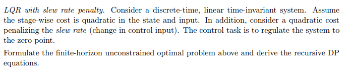
Give step-by-step solution with explanation and final answer:LQR with slew rate penalty. Consider a discrete-time, linear time-invariant system. Assume
the stage-wise cost is quadratic in the state a

Question

Give step-by-step solution with explanation and final answer:LQR with slew rate penalty. Consider a discrete-time, linear time-invariant system. Assume
the stage-wise cost is quadratic in the state and input. In addition, consider a quadratic cost
penalizing the slew rate (change in control input). The control task is to regulate the system to
the zero point.

Formulate the finite-horizon unconstrained optimal problem above and derive the recursive DP
equations.

VIPSolutions · Accepted Answer

Let's break down the problem and solve it **step by step**.

---

## 1. **System Dynamics**

Given a discrete-time, linear time-invariant (LTI) system:
$$
x_{k+1} = A x_k + B u_k
$$
where:
- $ x_k \in \mathbb{R}^n $: state at time $k$
- $ u_k \in \mathbb{R}^m $: control input

---

## 2. **Cost Function with Slew Rate Penalty**

The cost for each time step consists of:
- A quadratic penalty on state: $ x_k^T Q x_k $
- A quadratic penalty on control input: $ u_k^T R u_k $
- A quadratic penalty on the **slew rate** (change in control): $ (u_k - u_{k-1})^T S (u_k - u_{k-1}) $

Let the finite-horizon cost for horizon $N$ be:
$$
J = x_N^T Q_f x_N + \sum_{k=0}^{N-1} \left[
    x_k^T Q x_k + u_k^T R u_k + (u_k - u_{k-1})^T S (u_k - u_{k-1})
\right]
$$
where:
- $ Q \succeq 0, \, Q_f \succeq 0, \, R \succ 0, \, S \succeq 0 $
- $ u_{-1} $ is either given or assumed to be zero

---

## 3. **Augmented State Formulation**

The cost couples $ u_k $ and $ u_{k-1} $, so we **augment the state**:
Define
$$
z_k = \begin{bmatrix} x_k \ u_{k-1} \end{bmatrix}
$$
The augmented dynamics:
$$
z_{k+1} =
\begin{bmatrix}
    x_{k+1} \
    u_k
\end{bmatrix}
=
\begin{bmatrix}
    A x_k + B u_k \
    u_k
\end{bmatrix}
=
\begin{bmatrix}
    A & B \
    0 & 0
\end{bmatrix}
\begin{bmatrix}
    x_k \
    u_{k-1}
\end{bmatrix}
+
\begin{bmatrix}
    0 \
    I
\end{bmatrix}
u_k
$$
So:
$$
z_{k+1} = \underbrace{\begin{bmatrix} A & B \ 0 & 0 \end{bmatrix}}_{A_z} z_k + \underbrace{\begin{bmatrix} 0 \ I \end{bmatrix}}_{B_z} u_k
$$

---

## 4. **Augmented Cost Function**

Express the stage cost in terms of $ z_k $ and $ u_k $:

- $ x_k^T Q x_k = z_k^T \begin{bmatrix} Q & 0 \ 0 & 0 \end{bmatrix} z_k $
- $ u_k^T R u_k $
- $ (u_k - u_{k-1})^T S (u_k - u_{k-1}) = [u_k^T, u_{k-1}^T] \begin{bmatrix} S & -S \ -S & S \end{bmatrix} \begin{bmatrix} u_k \ u_{k-1} \end{bmatrix} $

So, the stage cost is:
$$
\ell(z_k, u_k) = z_k^T Q_z z_k + u_k^T R u_k + 
\begin{bmatrix} u_k \ u_{k-1} \end{bmatrix}^T
\begin{bmatrix} S & -S \ -S & S \end{bmatrix}
\begin{bmatrix} u_k \ u_{k-1} \end{bmatrix}
$$
But, using $ z_k = [x_k; u_{k-1}] $, and keeping only terms involving $ z_k $ and $ u_k $:

$$
\ell(z_k, u_k) = z_k^T \underbrace{\begin{bmatrix} Q & 0 \ 0 & S \end{bmatrix}}_{Q_z} z_k
+ u_k^T (R + S) u_k - 2 u_k^T S u_{k-1}
$$
or, in quadratic form:
$$
\ell(z_k, u_k) = \begin{bmatrix} z_k \ u_k \end{bmatrix}^T
\begin{bmatrix}
Q_z & -[0; S] \
-[0; S]^T & R+S
\end{bmatrix}
\begin{bmatrix}
z_k \ u_k
\end{bmatrix}
$$

---

## 5. **Finite-Horizon LQR Problem (Augmented)**

Formulate the problem as:
$$
\min_{\{u_k\}_{k=0}^{N-1}} z_N^T Q_{zf} z_N + \sum_{k=0}^{N-1} \left[
    z_k^T Q_z z_k + u_k^T (R + S) u_k - 2 u_k^T S u_{k-1}
\right]
$$
subject to:
$$
z_{k+1} = A_z z_k + B_z u_k
$$
with initial state $ z_0 = [x_0; u_{-1}] $.

---

## 6. **Dynamic Programming (DP) Recursion**

Assume the **value function** is quadratic:
$$
V_k(z_k) = z_k^T P_k z_k + 2 q_k^T z_k + r_k
$$

**Bellman recursion:**
$$
V_k(z_k) = \min_{u_k} \left\{ \ell(z_k, u_k) + V_{k+1}(z_{k+1}) \right\}
$$
with $ z_{k+1} = A_z z_k + B_z u_k $.

Substitute:
$$
V_k(z_k) = \min_{u_k} \left\{
    z_k^T Q_z z_k + u_k^T (R+S) u_k - 2 u_k^T S u_{k-1}
    + (A_z z_k + B_z u_k)^T P_{k+1} (A_z z_k + B_z u_k)
    + 2 q_{k+1}^T (A_z z_k + B_z u_k)
    + r_{k+1}
\right\}
$$

Group terms in $ u_k $:
$$
= \min_{u_k} \left\{
    u_k^T (R+S + B_z^T P_{k+1} B_z) u_k
    + 2 u_k^T (B_z^T P_{k+1} A_z z_k + B_z^T q_{k+1} - S u_{k-1})
    + z_k^T (Q_z + A_z^T P_{k+1} A_z) z_k
    + 2 q_{k+1}^T A_z z_k
    + r_{k+1}
\right\}
$$
Let:
$$
H = R+S + B_z^T P_{k+1} B_z
$$
$$
F = B_z^T P_{k+1} A_z
$$
$$
g = B_z^T q_{k+1} - S u_{k-1}
$$
The minimizer is:
$$
u_k^* = - H^{-1} (F z_k + g)
$$

---

## 7. **DP Recursion for Value Function**

Plug optimal $ u_k^* $ back into $ V_k(z_k) $:

$$
V_k(z_k) = z_k^T \left(Q_z + A_z^T P_{k+1} A_z - F^T H^{-1} F \right) z_k
+ 2 z_k^T \left(A_z^T q_{k+1} - F^T H^{-1} g \right)
+ r_{k+1} - g^T H^{-1} g
$$

Thus, the Riccati recursion is:
$$
P_k = Q_z + A_z^T P_{k+1} A_z - F^T H^{-1} F
$$
$$
q_k = A_z^T q_{k+1} - F^T H^{-1} g
$$
$$
r_k = r_{k+1} - g^T H^{-1} g
$$
with boundary condition $ P_N = Q_{zf} $, where $ Q_{zf} $ is the terminal cost.

---

## 8. **Final Answer: Summary**

### **Finite-horizon LQR with slew rate penalty:**

$$
\min_{\{u_k\}} \quad x_N^T Q_f x_N + \sum_{k=0}^{N-1} \left[
    x_k^T Q x_k + u_k^T R u_k + (u_k - u_{k-1})^T S (u_k - u_{k-1})
\right]
$$
subject to
$$
x_{k+1} = A x_k + B u_k
$$
with initial $ x_0 $, $ u_{-1} $.

### **Recursive DP Equations (in augmented state):**

Let $ z_k = \begin{bmatrix} x_k \ u_{k-1} \end{bmatrix} $, and define
$$
z_{k+1} = \begin{bmatrix} A & B \ 0 & 0 \end{bmatrix} z_k + \begin{bmatrix} 0 \ I \end{bmatrix} u_k
$$

The Riccati recursion is:
$$
P_k = Q_z + A_z^T P_{k+1} A_z - F^T H^{-1} F
$$
where
\[
Q_z = \begin{bmatrix} Q & 0 \ 0 & S \end{bmatrix}, \quad
A_z = \begin{bmatrix}

VIPSolutions · Answer

# Finite-Horizon LQR with Slew Rate Penalty: Formulation and DP Derivation

---

## 1. System Dynamics

Discrete-time, linear, time-invariant system:

$$
x_{k+1} = A x_k + B u_k
$$

- $x_k \in \mathbb{R}^n$: state
- $u_k \in \mathbb{R}^m$: control input

---

## 2. Cost Function

Stage-wise cost includes:

- Quadratic state penalty: $ x_k^T Q x_k $
- Quadratic input penalty: $ u_k^T R u_k $
- Quadratic slew rate penalty (change in input): $ (u_k - u_{k-1})^T S (u_k - u_{k-1}) $

Terminal cost:

$$
J = x_N^T Q_f x_N + \sum_{k=0}^{N-1} \left[
x_k^T Q x_k + u_k^T R u_k + (u_k - u_{k-1})^T S (u_k - u_{k-1})
\right]
$$

---

## 3. **Handling the Slew Rate Cost**

Since the cost couples $ u_k $ and $ u_{k-1} $, define **augmented state**:

$$
z_k = \begin{bmatrix} x_k \ u_{k-1} \end{bmatrix}
$$

- Initial $ u_{-1} $ is known or zero.

### Dynamics:

$$
\begin{bmatrix}
x_{k+1} \
u_k
\end{bmatrix}
= 
\underbrace{\begin{bmatrix}
A & B \
0 & 0
\end{bmatrix}}_{A_z}
z_k +
\underbrace{\begin{bmatrix}
0 \
I
\end{bmatrix}}_{B_z}
u_k
$$

---

## 4. **Cost in Terms of $z_k$ and $u_k$**

Express the stage cost:

$$
\ell(z_k, u_k) = x_k^T Q x_k + u_k^T R u_k + (u_k - u_{k-1})^T S (u_k - u_{k-1})
$$

In matrix form, using $ z_k = \begin{bmatrix} x_k \ u_{k-1} \end{bmatrix} $:

$$
\ell(z_k, u_k) = 
\begin{bmatrix} x_k \ u_{k-1} \ u_k \end{bmatrix}^T
\begin{bmatrix}
Q & 0 & 0 \
0 & S & -S \
0 & -S & S + R
\end{bmatrix}
\begin{bmatrix}
x_k \ u_{k-1} \ u_k
\end{bmatrix}
$$

Define:

$$
Q_z = \begin{bmatrix}
Q & 0 \
0 & S
\end{bmatrix}
$$

and the cross terms (see below). To keep the cost quadratic in $z_k$ and $ u_k $, the cost becomes:

$$
\ell(z_k, u_k) = z_k^T Q_z z_k + u_k^T (R + S) u_k - 2 u_k^T S u_{k-1}
$$

---

## 5. **Formulated Optimization Problem**

Minimize:

$$
J = x_N^T Q_f x_N + \sum_{k=0}^{N-1} \left[
z_k^T Q_z z_k + u_k^T (R+S) u_k - 2 u_k^T S u_{k-1}
\right]
$$

subject to:

$$
z_{k+1} = A_z z_k + B_z u_k
$$

---

## 6. **Dynamic Programming (DP) Approach**

Assuming quadratic value function:

$$
V_k(z_k) = z_k^T P_k z_k + 2 q_k^T z_k + r_k
$$

The **Bellman recursion**:

$$
V_k(z_k) = \min_{u_k} \left\{
\ell(z_k, u_k) + V_{k+1}(z_{k+1})
\right\}
$$

where:

$$
z_{k+1} = A_z z_k + B_z u_k
$$

---

## 7. **Optimal Control Law Derivation**

Express:

$$
V_{k+1}(z_{k+1}) = (A_z z_k + B_z u_k)^T P_{k+1} (A_z z_k + B_z u_k) + 2 q_{k+1}^T (A_z z_k + B_z u_k) + r_{k+1}
$$

Total cost:

$$
J_{total} = z_k^T Q_z z_k + u_k^T (R+S) u_k - 2 u_k^T S u_{k-1} + (A_z z_k + B_z u_k)^T P_{k+1} (A_z z_k + B_z u_k) + 2 q_{k+1}^T (A_z z_k + B_z u_k) + r_{k+1}
$$

---

## 8. **Quadratic Form in $ u_k $**

Group terms:

$$
J_{total} = u_k^T H u_k + 2 u_k^T F z_k + \text{(terms in } z_k \text{ only)}
$$

where:

$$
H = R + S + B_z^T P_{k+1} B_z
$$

$$
F = B_z^T P_{k+1} A_z + B_z^T q_{k+1}
$$

The cross-term with $ u_{k-1} $:

$$
- 2 u_k^T S u_{k-1}
$$

This acts as a linear term in $ u_k $ with coefficient dependent on $ u_{k-1} $.

---

## 9. **Optimal Control Input**

The optimal $ u_k $:

$$
u_k^* = - H^{-1} \left( F z_k - S u_{k-1} \right)
$$

which includes the previous control $ u_{k-1} $.

---

## 10. **Recursion for Value Function**

The value function is quadratic:

$$
P_k = Q_z + A_z^T P_{k+1} A_z - F^T H^{-1} F
$$

with:

$$
F = B_z^T P_{k+1} A_z + B_z^T q_{k+1}
$$

and the cross term involving $ u_{k-1} $:

$$
g_k = - S u_{k-1}
$$

The updated value function parameters are:

$$
q_k = A_z^T q_{k+1} - F^T H^{-1} g_k
$$

$$
r_k = r_{k+1} - g_k^T H^{-1} g_k
$$

---

## **Summary**

### **Problem formulation:**

$$
\boxed{
\begin{aligned}
&\text{Minimize} \quad J = x_N^T Q_f x_N + \sum_{k=0}^{N-1} \left[
x_k^T Q x_k + u_k^T R u_k + (u_k - u_{k-1})^T S (u_k - u_{k-1})
\right] \
&\text{Subject to} \quad x_{k+1} = A x_k + B u_k
\end{aligned}
}
$$

### **DP recursive equations:**

- **Augmented state:**

$$
z_k = \begin{bmatrix} x_k \ u_{k-1} \end{bmatrix}
$$

- **Dynamics:**

$$
z_{k+1} = A_z z_k + B_z u_k,\quad
A_z = \begin{bmatrix} A & B \ 0 & 0 \end{bmatrix}, \quad B_z = \begin{bmatrix} 0 \ I \end{bmatrix}
$$

- **Cost matrices:**

$$
Q_z = \begin{bmatrix} Q & 0 \ 0 & S \end{bmatrix}
$$

- **Riccati recursion:**

$$
P_k = Q_z + A_z^T P_{k+1} A_z - \left(B_z^T P_{k+1} A_z + B_z^T q_{k+1}\right)^T H^{-1} \left(B_z^T P_{k+1} A_z + B_z^T q_{k+1}\right)
$$

where:

$$
H = R + S + B_z^T P_{k+1} B_z
$$

- **Control law:**

$$
u_k^* = - H^{-1} \left( B_z^T P_{k+1} A_z z_k + B_z^T q_{k+1} - S u_{k-1} \right)
$$

---

This derivation provides the framework for implementing an optimal control policy penalizing both control effort and slew rate change over a finite horizon.

✨ VIPSolutions

Question:

Final Answer:

Question:

Final Answer:

📢 Instructions:

Study Help, Fast Answers

✨ VIPSolutions

Question:

Final Answer:

Question:

Final Answer:

📢 Instructions:

Related Answers

Study Help, Fast Answers