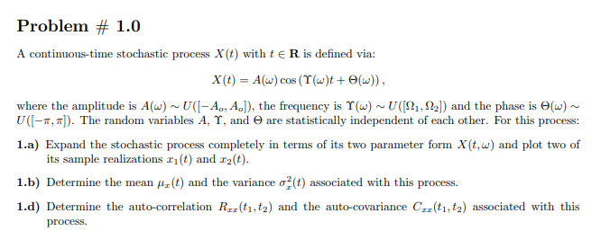
Let's solve the given problem step by step. --- ## **Given:** A continuous-time stochastic process \( X(t) \) defined as: \[ X(t) = A(\omega) \cos(\Upsilon(\omega)t + \Theta(\omega)) \] where: - \( A(\omega) \sim \mathcal{U}([-A_0, A_0]) \) (Uniform distribution) - \( \Upsilon(\omega) \sim \mathcal{U}([\Omega_1, \Omega_2]) \) (Uniform distribution) - \( \Theta(\omega) \sim \mathcal{U}([-\pi, \pi]) \) (Uniform distribution) - \( A, \Upsilon, \Theta \) are independent. --- ## **1.a) Expand \( X(t) \) in terms of \( X(t, \omega) \) and plot two sample realizations** ### **Expansion:** The process is already written as: \[ X(t, \omega) = A(\omega) \cos(\Upsilon(\omega) t + \Theta(\omega)) \] **Sample realizations:** To plot two sample realizations, pick two sets of random values \((A_1, \Upsilon_1, \Theta_1)\) and \((A_2, \Upsilon_2, \Theta_2)\): - \( x_1(t) = A_1 \cos(\Upsilon_1 t + \Theta_1) \) - \( x_2(t) = A_2 \cos(\Upsilon_2 t + \Theta_2) \) **For example:** - Let \( A_1 = 1 \), \( \Upsilon_1 = 2 \), \( \Theta_1 = 0 \) - Let \( A_2 = -0.5 \), \( \Upsilon_2 = 1 \), \( \Theta_2 = \pi/4 \) So, - \( x_1(t) = \cos(2t) \) - \( x_2(t) = -0.5 \cos(t + \pi/4) \) (You can plot these using any plotting tool.) --- ## **1.b) Mean \( \mu_X(t) \) and Variance \( \sigma_X^2(t) \)** ### **Mean:** \[ \mu_X(t) = \mathbb{E}[X(t)] = \mathbb{E}[A] \cdot \mathbb{E}[\cos(\Upsilon t + \Theta)] \] \( \mathbb{E}[A] = 0 \) (since \( A \) is uniform over symmetric interval) \[ \mathbb{E}[\cos(\Upsilon t + \Theta)] = 0 \quad \text{(since expectation over uniform phase on } [-\pi, \pi] \text{ is zero)} \] So, \[ \boxed{\mu_X(t) = 0} \] ### **Variance:** \[ \sigma_X^2(t) = \mathbb{E}[X(t)^2] - (\mathbb{E}[X(t)])^2 = \mathbb{E}[X(t)^2] \] Since \( \mathbb{E}[X(t)] = 0 \): \[ X(t)^2 = A^2 \cos^2(\Upsilon t + \Theta) \] So, \[ \mathbb{E}[X(t)^2] = \mathbb{E}[A^2] \cdot \mathbb{E}[\cos^2(\Upsilon t + \Theta)] \] - \( \mathbb{E}[A^2] = \frac{A_0^2}{3} \) (for uniform over \([-A_0, A_0]\)) - \( \mathbb{E}[\cos^2(\cdot)] = \frac{1}{2} \) (since uniform on phase over full period) So, \[ \sigma_X^2(t) = \frac{A_0^2}{3} \cdot \frac{1}{2} = \boxed{\frac{A_0^2}{6}} \] --- ## **1.d) Auto-correlation \( R_{xx}(t_1, t_2) \) and Auto-covariance \( C_{xx}(t_1, t_2) \)** ### **Auto-correlation:** \[ R_{xx}(t_1, t_2) = \mathbb{E}[X(t_1) X(t_2)] \] \[ = \mathbb{E}\left[ A^2 \cos(\Upsilon t_1 + \Theta) \cos(\Upsilon t_2 + \Theta) \right] \] \[ = \mathbb{E}[A^2] \cdot \mathbb{E}\left[ \cos(\Upsilon t_1 + \Theta) \cos(\Upsilon t_2 + \Theta) \right] \] Recall: \[ \cos a \cos b = \frac{1}{2} [\cos(a-b) + \cos(a+b)] \] Let \( a = \Upsilon t_1 + \Theta \), \( b = \Upsilon t_2 + \Theta \): \[ = \mathbb{E}[A^2] \cdot \frac{1}{2} \mathbb{E}\left[ \cos(\Upsilon (t_1 - t_2)) + \cos(\Upsilon (t_1 + t_2) + 2\Theta) \right] \] Since \( \Theta \) is uniform over \([-\pi, \pi]\), \( \mathbb{E}[\cos(\Upsilon (t_1 + t_2) + 2\Theta)] = 0 \). So, \[ R_{xx}(t_1, t_2) = \mathbb{E}[A^2] \cdot \frac{1}{2} \mathbb{E}[\cos(\Upsilon (t_1 - t_2))] \] With \( \mathbb{E}[A^2] = \frac{A_0^2}{3} \): \[ R_{xx}(t_1, t_2) = \frac{A_0^2}{6} \mathbb{E}_{\Upsilon}[\cos(\Upsilon (t_1 - t_2))] \] If \( \Upsilon \sim \mathcal{U}([\Omega_1, \Omega_2]) \): \[ \mathbb{E}_{\Upsilon}[\cos(\Upsilon \tau)] = \frac{1}{\Omega_2 - \Omega_1} \int_{\Omega_1}^{\Omega_2} \cos(\Upsilon \tau) d\Upsilon \] \[ = \frac{1}{\Omega_2 - \Omega_1} \left[ \frac{\sin(\Upsilon \tau)}{\tau} \right]_{\Omega_1}^{\Omega_2} = \frac{1}{\Omega_2 - \Omega_1} \cdot \frac{\sin(\Omega_2 \tau) - \sin(\Omega_1 \tau)}{\tau} \] where \( \tau = t_1 - t_2 \). So, \[ \boxed{ R_{xx}(t_1, t_2) = \frac{A_0^2}{6} \cdot \frac{\sin(\Omega_2 (t_1-t_2)) - \sin(\Omega_1 (t_1-t_2))}{(\Omega_2 - \Omega_1)(t_1-t_2)} } \] ### **Auto-covariance:** \[ C_{xx}(t_1, t_2) = R_{xx}(t_1, t_2) - \mu_X(t_1)\mu_X(t_2) \] But \( \mu_X(t) = 0 \), so, \[ \boxed{C_{xx}(t_1, t_2) = R_{xx}(t_1, t_2)} \] --- ## **Summary of Answers** ### **1.a** \[ X(t, \omega) = A(\omega) \cos(\Upsilon(\omega) t + \Theta(\omega)) \] Sample realizations: \( x_1(t) \), \( x_2(t) \) as above. ### **1.b** \[ \mu_X(t) = 0, \quad \sigma_X^2(t) = \frac{A_0^2}{6} \] ### **1.d** \[ R_{xx}(t_1, t_2) = \frac{A_0^2}{6} \cdot \frac{\sin(\Omega_2 (t_1-t_2)) - \sin(\Omega_1 (t_1-t_2))}{(\Omega_2 - \Omega_1)(t_1-t_2)} \] \[ C_{xx}(t_1, t_2) = R_{xx}(t_1, t_2) \] Let me know if you need the plots or further explanation!

1.a) The process \(X(t, \omega) = A(\omega)\cos(\Upsilon(\omega)t + \Theta(\omega))\), with independent uniformly distributed amplitude, frequency, and phase, can be realized by sampling these variables and plotting the resulting cosine functions for different realizations. 1.b) The mean \( \mu_X(t) \) is zero, since the average of the symmetric uniform phase cancels out. Variance \( \sigma_X^2(t) \) is \( A_0^2/6 \), derived from the second moment of the amplitude and phase independence. 1.d) The autocorrelation \( R_{xx}(t_1,t_2) \) depends on the expected cosine of frequency times time difference, resulting in a sinc-like function. The autocovariance equals the autocorrelation as the mean is zero, reflecting the process's second-order properties.