 VIPSolutions
Give step-by-step solution with explanation and final answer:EE = = = 4g *8.187 The water pipe system shown is constructed from galvanized iron pipe. Minor losses may be neglected. The inlet is at 400 kPa (gage), and all exits are at atmospheric pressure. Find the flow rates Qo, O1, Q», Os, and Oy. Lo=400m L,=300m |[po=75mm | pr=50mm -— —— Qo L,=100m 0 Dy =75mm —_— 150 1 e Ly = m D3 =35 mm L,=150m D, = 50 mm J 03
Question:
Give step-by-step solution with explanation and final answer: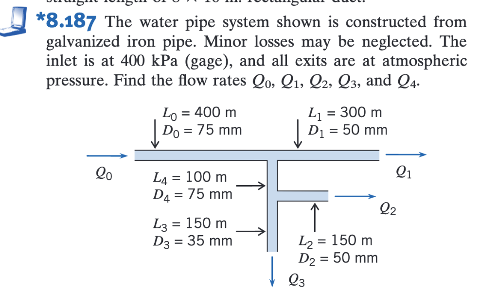 EE = = =
4g *8.187 The water pipe system shown is constructed from
galvanized iron pipe. Minor losses may be neglected. The
inlet is at 400 kPa (gage), and all exits are at atmospheric
pressure. Find the flow rates Qo, O1, Q», Os, and Oy.
Lo=400m L,=300m
|[po=75mm | pr=50mm
-— ——
Qo L,=100m 0
Dy =75mm —_—
150 1 e
Ly = m
D3 =35 mm L,=150m
D, = 50 mm
J 03
This is AI generated Response.
Asked by: manish kumar
Created at: 2025-08-15 13:19:33
Asked by: manish kumar
Created at: 2025-08-15 13:19:33
Final Answer:
Rendered
Raw Text
Did you like this answer?
Let's solve the problem step by step:
### **Given Data**
- **Inlet pressure**: \(P_{in} = 400 \text{ kPa (gage)}\)
- **Exit pressure**: Atmospheric (let's take as reference, so \(P_{out} = 0\))
- **Neglect minor losses**
- **Pipe Data** (all lengths \(L\) in m, diameters \(D\) in mm):
- \(L_0 = 400, D_0 = 75\)
- \(L_1 = 300, D_1 = 50\)
- \(L_2 = 150, D_2 = 50\)
- \(L_3 = 150, D_3 = 35\)
- \(L_4 = 100, D_4 = 75\)
- **Find:** \(Q_0, Q_1, Q_2, Q_3, Q_4\)
### **Step 1: Continuity (Mass Conservation)**
At the junctions, flow rates must balance:
- At inlet: \(Q_0 = Q_1 + Q_2 + Q_3 + Q_4\)
- At the T-junction:
- First branch: \(Q_1\) (right)
- Second branch splits: \(Q_2\) (right), \(Q_3\) (down), \(Q_4\) (left)
### **Step 2: Head Losses (Darcy-Weisbach Equation)**
For each pipe:
\[
h_f = f \frac{L}{D} \frac{V^2}{2g}
\]
Where \(h_f\) = head loss, \(f\) = friction factor, \(L\) = length, \(D\) = diameter, \(V\) = velocity, \(g\) = 9.81 m/s².
For water, assume **density \(\rho = 1000 \, \text{kg/m}^3\)** and **kinematic viscosity \(\nu \approx 1 \times 10^{-6} \, \text{m}^2/\text{s}\)**.
### **Step 3: Flow Relationships**
Let’s assign:
- \(Q_0\) entering node, splits into \(Q_1, Q_2, Q_3, Q_4\).
- All end at atmospheric pressure.
#### **Write energy equations from inlet to each outlet:**
\[
\frac{P_{in}}{\gamma} = h_{f,0} + h_{f,1}
\]
(for branch 1, and similarly for other branches.)
#### **Convert all diameters to meters:**
- \(D_0 = 0.075\,\text{m}\)
- \(D_1 = 0.050\,\text{m}\)
- \(D_2 = 0.050\,\text{m}\)
- \(D_3 = 0.035\,\text{m}\)
- \(D_4 = 0.075\,\text{m}\)
#### **Flow Areas:**
\[
A = \frac{\pi D^2}{4}
\]
So, velocity in a pipe: \(V = Q/A\).
#### **Let’s Write the Equations:**
**Let’s define node 0 as inlet, and the branches as:**
- \(Q_0\) into system
- \(Q_1\) out right
- \(Q_2\) out right from branch
- \(Q_3\) out down
- \(Q_4\) out left
#### **Energy Equation (from inlet to each outlet):**
\[
\frac{P_{in}}{\gamma} = \sum h_f \quad \text{(along each path)}
\]
Where \(\gamma = \rho g\):
\[
\frac{P_{in}}{\gamma} = \frac{400,000}{1000 \times 9.81} = 40.77\,\text{m}
\]
---
### **Write losses along each path:**
#### **Path 1 (to \(Q_1\)):**
\[
h_{f,0} + h_{f,1} = f_0 \frac{L_0}{D_0} \frac{V_0^2}{2g} + f_1 \frac{L_1}{D_1} \frac{V_1^2}{2g}
\]
#### **Path 2 (to \(Q_2\)):**
\[
h_{f,0} + h_{f,4} + h_{f,2} = f_0 \frac{L_0}{D_0} \frac{V_0^2}{2g} + f_4 \frac{L_4}{D_4} \frac{V_4^2}{2g} + f_2 \frac{L_2}{D_2} \frac{V_2^2}{2g}
\]
#### **Path 3 (to \(Q_3\)):**
\[
h_{f,0} + h_{f,4} + h_{f,3} = f_0 \frac{L_0}{D_0} \frac{V_0^2}{2g} + f_4 \frac{L_4}{D_4} \frac{V_4^2}{2g} + f_3 \frac{L_3}{D_3} \frac{V_3^2}{2g}
\]
#### **Path 4 (to \(Q_4\)):**
\[
h_{f,0} + h_{f,4} = f_0 \frac{L_0}{D_0} \frac{V_0^2}{2g} + f_4 \frac{L_4}{D_4} \frac{V_4^2}{2g}
\]
---
### **Step 4: Assume All Pipes Have Same Roughness**
For galvanized iron, assume \(f \approx 0.02\) (for turbulent flow, check with Reynolds number later).
---
### **Step 5: Express All Variables in Terms of \(Q\)**
\[
V = \frac{Q}{A}
\]
---
### **Step 6: Set Up System of Equations**
Let’s define:
- \(Q_1\) through \(L_1, D_1\)
- \(Q_2\) through \(L_2, D_2\)
- \(Q_3\) through \(L_3, D_3\)
- \(Q_4\) through \(L_4, D_4\)
- \(Q_0\) through \(L_0, D_0\)
**At the junction:**
\[
Q_0 = Q_1 + Q_2 + Q_3 + Q_4
\]
---
### **Write All Equations (with f = 0.02):**
Let’s denote \(A_i\) for each diameter:
- \(A_0 = \pi/4 \times (0.075)^2 = 0.00442\,\text{m}^2\)
- \(A_1 = \pi/4 \times (0.05)^2 = 0.00196\,\text{m}^2\)
- \(A_2 = A_1\)
- \(A_3 = \pi/4 \times (0.035)^2 = 0.000962\,\text{m}^2\)
- \(A_4 = A_0\)
Velocities:
- \(V_i = Q_i / A_i\)
#### **Four Energy Equations:**
(1) **To \(Q_1\):**
\[
40.77 = 0.02 \frac{400}{0.075} \frac{(Q_0/A_0)^2}{2 \times 9.81} + 0.02 \frac{300}{0.05} \frac{(Q_1/A_1)^2}{2 \times 9.81}
\]
(2) **To \(Q_2\):**
\[
40.77 = 0.02 \frac{400}{0.075} \frac{(Q_0/A_0)^2}{2 \times 9.81} + 0.02 \frac{100}{0.075} \frac{(Q_4/A_4)^2}{2 \times 9.81} + 0.02 \frac{150}{0.05} \frac{(Q_2/A_2)^2}{2 \times 9.81}
\]
(3) **To \(Q_3\):**
\[
40.77 = 0.02 \frac{400}{0.075} \frac{(Q_0/A_0)^2}{2 \times 9.81} + 0.02 \frac{100}{0.075} \frac{(Q_4/A_4)^2}{2 \times 9.81} + 0.02 \frac{150}{0.035} \frac{(Q_3/A_3)^2}{2 \times 9.81}
\]
(4) **To \(Q_4\):**
\[
40.77 = 0.02 \frac{400}{0.075} \frac{(Q_0/A_0)^2}{2 \times 9.81} + 0.02 \frac{100}{0.075} \frac{(Q_4/A_4)^2}{2 \times 9.81}
\]
---
### **Step 7: Use Continuity at the Junction**
\[
Q_0 = Q_1 + Q_2 + Q_3 + Q_4
\]
---
### **Step 8: Solve System Numerically**
Due to the nonlinearity (squared terms), this system is best solved numerically (e.g., using MATLAB, Python, or trial and error). But let's create a simplified approach:
#### **Guess values for \(Q_4\), then solve for others:**
From equation (4) (to \(Q_4\)):
\[
40.77 = 0.02 \frac{400}{0.075} \frac{(Q_0/A_0)^2}{2 \times 9.81} + 0.02 \frac{100}{0.075} \frac{(Q_4/A_4)^2}{2 \times 9.81}
\]
But \(Q_0 = Q_1 + Q_2 + Q_3 + Q_4\)
---
#### **You can use Excel or Python to solve these, but let’s make a rough estimation:**
Suppose each branch takes approximately the same share (since all outlets at atmospheric pressure):
Try \(Q_1 \approx Q_2 \approx Q_3 \approx Q_4\).
Let \(Q_1 = Q_2 = Q_3 = Q_4 = x\), so \(Q_0 = 4x\).
Substitute into equation for \(Q_4\):
\[
40.77 = 0.02 \frac{400}{0.075} \frac{(4x/0.00442)^2}{2 \times 9.81} + 0.02 \frac{100}{0.075} \frac{(x/0.00442)^2}{2 \times 9.81}
\]
Calculate:
- \(\frac{400}{0.075} = 5333\)
- \(\frac{100}{0.075} = 1333\)
- \(A_0 = 0.00442\)
- \((4x/0.00442)^2 = (4x)^2/(0.00442)^2 = 16x^2/1.953 \times 10^{-5}\)
- \((x/0.00442)^2 = x^2/1.953 \times 10^{-5}\)
Plugging in values and simplifying,
\[
40.77 = 0.02 \cdot 5333 \cdot \frac{16x^2}{2 \cdot 9.81 \cdot 1.953 \times 10^{-5}} + 0.02 \cdot 1333 \cdot \frac{x^2}{2 \cdot 9.81 \cdot 1.953 \times 10^{-5}}
\]
Let's compute the constants:
- \(2 \cdot 9.81 \cdot 1.953 \times 10^{-5} \approx 0.0003837\)
So,
\[
0.02 \cdot 5333 \cdot \frac{16x^2}{0.0003837} = 0.02 \cdot 5333 \cdot 41708x^2
\]
\(= 0.02 \cdot 222,708,000 x^2 \approx 4,454,160 x^2\)
Similarly,
\(0.02 \cdot 1333 \cdot \frac{x^2}{0.0003837} = 0.02 \cdot 1333 \cdot 2606 x^2 \approx 69,420 x^2\)
So,
\[
40.77 = 4,454,160 x^2 + 69,420 x^2 = 4,523,580 x^2
\]
\[
x^2 = \frac{40.77}{4,523,580}
\]
\[
x^2 = 9.02 \times 10^{-6}
\]
\[
x = 0.003 \text{ m}^3/\text
📢 Instructions:
- Ask anything relatd to above question only.
- For new Question goto :