 VIPSolutions
Give step-by-step solution with explanation and final answer:Let Xi = Zy + 2211 — 8%». i Identify the model as MA(q) or AR(p), specify q or p respectively. ii Is the model stationary and invertible? Explain fully and show calculations where needed. iii Find py (2). iv Write an R script (to be submitted and required to be commented) that will simulate 300 values of {X:} and use these simulated values to plot sample acf. Compare your sample estimate of px (2) to its true value found by calculations. Redo this part using 10,000 simulated values of X;. Comment on findings.
Question:
Give step-by-step solution with explanation and final answer: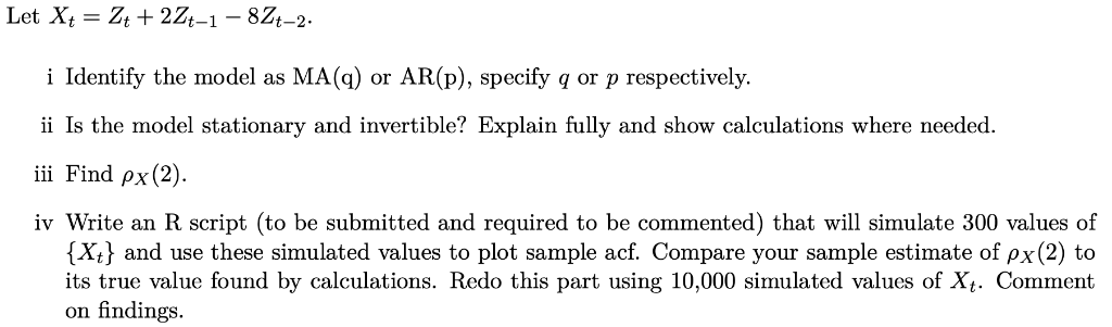 Let Xi = Zy + 2211 — 8%».
i Identify the model as MA(q) or AR(p), specify q or p respectively.
ii Is the model stationary and invertible? Explain fully and show calculations where needed.
iii Find py (2).
iv Write an R script (to be submitted and required to be commented) that will simulate 300 values of
{X:} and use these simulated values to plot sample acf. Compare your sample estimate of px (2) to
its true value found by calculations. Redo this part using 10,000 simulated values of X;. Comment
on findings.
This is AI generated Response.
Asked by: Umesh
Created at: 2025-07-26 23:23:49
Asked by: Umesh
Created at: 2025-07-26 23:23:49
Final Answer:
Rendered
Raw Text
Did you like this answer?
Let's solve each part step by step:
---
### (i) **Identify the model as MA(q) or AR(p), specify q or p respectively.**
Given:
\[ X_t = Z_t + 2Z_{t-1} - 8Z_{t-2} \]
This is a linear combination of current and past white noise terms (\( Z_t \)), which fits the definition of a **Moving Average (MA)** model.
The general form for MA(q):
\[
X_t = Z_t + \theta_1 Z_{t-1} + \theta_2 Z_{t-2} + \cdots + \theta_q Z_{t-q}
\]
Comparing, we have nonzero coefficients up to \( Z_{t-2} \). So, **q = 2**.
**Answer:**
The model is **MA(2)**.
---
### (ii) **Is the model stationary and invertible? Explain fully and show calculations where needed.**
#### **Stationarity**
MA(q) models are **always stationary** because they are a finite linear combination of white noise terms.
#### **Invertibility**
For invertibility, the roots of the MA polynomial must lie **outside the unit circle**.
The MA polynomial is:
\[
\theta(B) = 1 + 2B - 8B^2
\]
Set \(\theta(B) = 0\):
\[
1 + 2B - 8B^2 = 0 \implies 8B^2 - 2B - 1 = 0
\]
Solve for \(B\):
\[
B = \frac{2 \pm \sqrt{(-2)^2 - 4 \cdot 8 \cdot (-1)}}{2 \cdot 8}
= \frac{2 \pm \sqrt{4 + 32}}{16}
= \frac{2 \pm 6}{16}
\]
So,
- \(B_1 = \frac{2+6}{16} = \frac{8}{16} = 0.5\)
- \(B_2 = \frac{2-6}{16} = \frac{-4}{16} = -0.25\)
These roots are **inside** the unit circle (since \(|0.5| < 1\) and \(|-0.25| < 1\)), so the model is **not invertible**.
**Answer:**
- The model is **stationary** (all MA models are).
- The model is **not invertible** because the roots of the MA polynomial are inside the unit circle.
---
### (iii) **Find \(\rho_X(2)\) (the autocorrelation at lag 2).**
Recall for MA(2):
\[
X_t = Z_t + \theta_1 Z_{t-1} + \theta_2 Z_{t-2}
\]
Here, \(\theta_1 = 2\), \(\theta_2 = -8\).
The general autocovariance formula for MA(2) (assuming \(Z_t\) is white noise with variance \(\sigma^2\)):
- \(\gamma_X(0) = (1^2 + \theta_1^2 + \theta_2^2)\sigma^2\)
- \(\gamma_X(1) = (1 \cdot \theta_1 + \theta_1 \cdot \theta_2)\sigma^2\)
- \(\gamma_X(2) = (1 \cdot \theta_2)\sigma^2\)
- For \(h > 2\), \(\gamma_X(h) = 0\)
So,
\[
\gamma_X(0) = (1^2 + 2^2 + (-8)^2)\sigma^2 = (1+4+64)\sigma^2 = 69\sigma^2
\]
\[
\gamma_X(2) = (1 \cdot -8)\sigma^2 = -8\sigma^2
\]
\[
\rho_X(2) = \frac{\gamma_X(2)}{\gamma_X(0)} = \frac{-8\sigma^2}{69\sigma^2} = -\frac{8}{69}
\]
**Final Answer:**
\[
\rho_X(2) = -\frac{8}{69} \approx -0.116
\]
---
### (iv) **Write an R script...**
Below is an R script that simulates \(X_t\) for 300 and 10,000 values, computes sample acf, and compares \(\rho_X(2)\):
```r
# (a) Simulate MA(2) process
set.seed(123) # for reproducibility
# Function to simulate and analyze
analyze_MA2 <- function(n) {
Z <- rnorm(n + 2) # extra 2 for lag
X <- Z[3:(n+2)] + 2 * Z[2:(n+1)] - 8 * Z[1:n]
# Plot sample acf
acf(X, main = paste("Sample ACF (n =", n, ")"))
# Sample autocorrelation at lag 2
acf_values <- acf(X, plot = FALSE)$acf
sample_rho2 <- acf_values[3] # lag 2 is third value (lags: 0,1,2)
cat("Sample rho_X(2) for n =", n, ":", sample_rho2, "\n")
return(sample_rho2)
}
# (b) For n = 300
sample_rho2_300 <- analyze_MA2(300)
cat("Theoretical rho_X(2):", -8/69, "\n")
# (c) For n = 10,000
sample_rho2_10000 <- analyze_MA2(10000)
# Compare
cat("Sample rho_X(2) with n = 300:", sample_rho2_300, "\n")
cat("Sample rho_X(2) with n = 10000:", sample_rho2_10000, "\n")
cat("Theoretical rho_X(2):", -8/69, "\n")
```
#### **Comments on findings:**
- With \(n = 300\), the sample autocorrelation at lag 2 (\(\rho_X(2)\)) may deviate from the theoretical value due to sampling variability.
- With \(n = 10,000\), the sample autocorrelation should be much closer to the theoretical value (\(-8/69 \approx -0.116\)), illustrating the law of large numbers.
---
## **Summary of answers**
**(i)** MA(2) model
**(ii)** Stationary but not invertible
**(iii)** \(\rho_X(2) = -\frac{8}{69} \approx -0.116\)
**(iv)** See R code above; larger sample sizes yield sample autocorrelations closer to the theoretical value.
📢 Instructions:
- Ask anything relatd to above question only.
- For new Question goto :