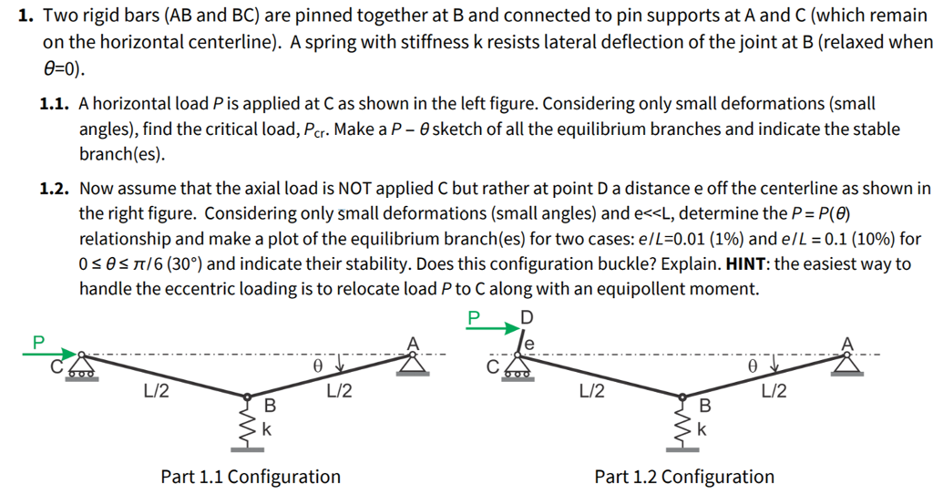
Give step-by-step solution with explanation and final answer:1. Two rigid bars (AB and BC) are pinned together at B and connected to pin supports at A and C (which remain
on the horizontal centerline). A spring with stiffness k resists lateral deflection of the joint at B (relaxed when
6-0).
1.1. Ahorizontal load Pis applied at C as shown in the left figure. Considering only small deformations (small
angles), find the critical load, Pc. Make a P — 8 sketch of all the equilibrium branches and indicate the stable
branch(es).
1.2. Now assume that the axial load is NOT applied C but rather at point D a distance e off the centerline as shown in
the right figure. Considering only small deformations (small angles) and e
Question:
Give step-by-step solution with explanation and final answer:1. Two rigid bars (AB and BC) are pinned together at B and connected to pin supports at A and C (which remain
on the horizontal centerline). A spring with stiffness k resists lateral deflection of the joint at B (relaxed when
6-0).
1.1. Ahorizontal load Pis applied at C as shown in the left figure. Considering only small deformations (small
angles), find the critical load, Pc. Make a P — 8 sketch of all the equilibrium branches and indicate the stable
branch(es).
1.2. Now assume that the axial load is NOT applied C but rather at point D a distance e off the centerline as shown in
the right figure. Considering only small deformations (small angles) and e
This is AI generated Response.
Asked by: gvr
Created at: 2025-07-04 11:56:06
Final Answer:
RenderedRaw Text
Did you like this answer?
Let's solve each part step by step:
---
## **1.1. Find the Critical Load \( P_{cr} \) for the Symmetric Case**
### **Step 1: Draw the Free Body Diagram and Write Equilibrium**
- The load \( P \) is applied horizontally at \( C \).
- The bars \( AB \) and \( BC \) are rigid and pinned at \( B \).
- There's a spring of stiffness \( k \) at \( B \).
When a small angle \( \theta \) is formed, the joint \( B \) is displaced vertically by \( y_B \approx (L/2)\sin\theta \approx (L/2)\theta \) (for small angles).
#### **Moment Equilibrium about B:**
The spring force at \( B \) is \( F_s = k y_B = k (L/2)\theta \).
The horizontal force \( P \) at \( C \) creates a moment at \( B \) about the centerline:
\[
\text{Moment from } P: \quad M_P = P \times \text{vertical distance from B to C}
\]
For small \( \theta \), the vertical displacement of \( C \) is approximately:
\[
\Delta y_C = (L) \sin\theta \approx L\theta
\]
But \( C \) is pinned and can't move vertically. Instead, consider the moment arm from \( B \) to \( C \), which is \( (L/2) \sin\theta \approx (L/2)\theta \):
\[
\text{Moment from } P = P \times (L/2)\theta
\]
#### **Set up the Equilibrium Equation:**
Sum of moments at \( B \):
\[
M_P - F_s \times (L/2) = 0
\]
\[
P \times (L/2)\theta - k (L/2)\theta = 0
\]
\[
(P - k) \frac{L}{2}\theta = 0
\]
For nontrivial solutions (\(\theta \neq 0\)):
\[
P_{cr} = k
\]
---
### **Step 2: \( P-\theta \) Equilibrium Path and Stability**
- For \( P < k \): Only solution is \( \theta = 0 \) (stable).
- For \( P = k \): \(\theta = 0\) is a bifurcation point; nontrivial solutions emerge.
- For \( P > k \): Nontrivial solutions exist, but they are unstable (spring cannot restore the displacement).
#### **Sketch:**
- \( P \) on the y-axis, \( \theta \) on the x-axis.
- Stable branch: Horizontal line at \( \theta = 0 \) for \( P < k \).
- At \( P = k \), a pitchfork bifurcation (critical load).
- For \( P > k \), branches at \(\pm\theta\), both unstable.
---
## **1.2. Eccentric Loading at D (Off Centerline)**
### **Given:**
- Load \( P \) at point \( D \), distance \( e \) above \( C \).
### **Step 1: Replace Load with Equivalent System**
Move \( P \) at \( D \) to \( C \), but add a moment \( M = P \cdot e \) at \( C \) **(as per the hint).**
### **Step 2: Moment Equilibrium about B**
- Load \( P \) at \( C \) as before.
- Additional **moment** at \( C \) (or at B, since B is at the center of the structure): \( M = P e \).
The moment equilibrium at B becomes:
\[
P \cdot (L/2)\theta + P e - k (L/2)\theta = 0
\]
\[
(P - k) \frac{L}{2}\theta + P e = 0
\]
\[
(P - k) \frac{L}{2}\theta = -P e
\]
\[
(P - k)\theta = -\frac{2Pe}{L}
\]
\[
P\theta - k\theta + \frac{2Pe}{L} = 0
\]
\[
P\theta + \frac{2Pe}{L} = k\theta
\]
\[
P\theta - k\theta = -\frac{2Pe}{L}
\]
\[
\theta(P-k) = -\frac{2Pe}{L}
\]
\[
\theta = -\frac{2Pe}{L(P-k)}
\]
---
### **Step 3: Find \( P(\theta) \) Relation**
\[
\theta = -\frac{2Pe}{L(P-k)}
\]
\[
-\theta (P-k) = \frac{2Pe}{L}
\]
\[
-\theta P + \theta k = \frac{2Pe}{L}
\]
\[
-\theta P - \frac{2Pe}{L} = -\theta k
\]
\[
P(-\theta - \frac{2e}{L}) = -\theta k
\]
\[
P = \frac{-\theta k}{-\theta - \frac{2e}{L}}
\]
\[
P = \frac{\theta k}{\theta + \frac{2e}{L}}
\]
---
### **Step 4: Plot \( P = P(\theta) \) for Given \( e/L \) Values**
For small \( e \):
#### **Case 1: \( e/L = 0.01 \)**
\[
P = \frac{\theta k}{\theta + 0.02}
\]
#### **Case 2: \( e/L = 0.1 \)**
\[
P = \frac{\theta k}{\theta + 0.2}
\]
---
### **Stability and Buckling**
- With eccentricity, the trivial solution (\( \theta = 0 \)) no longer exists for any \( P \neq 0 \).
- **No bifurcation/buckling:** The system responds smoothly for all \( P \); there is no sudden jump.
- The load-deformation path is *smooth*, not a bifurcation (buckling) as with \( e = 0 \).
---
### **Summary Table**
| Case | Equation | Buckling? | Stable? |
|--------------|----------------------------------|-----------|-------------|
| \( e = 0 \) | \( P_{cr} = k \) | Yes | Stable for \( P < k \) |
| \( e \neq 0 \)| \( P = \frac{\theta k}{\theta + 2e/L} \) | No | Single stable path |
---
## **Final Answers**
### **1.1.**
- **Critical load:** \( \boxed{P_{cr} = k} \)
- **Sketch:** Pitchfork bifurcation at \( P = k \).
### **1.2.**
- **Equilibrium path:** \( \boxed{P = \frac{\theta k}{\theta + 2e/L}} \)
- **No buckling**: The system does *not* buckle for \( e \neq 0 \); it follows a smooth equilibrium path.
- **Stability:** The system is stable for all \( P \).
---
#### **Sample Sketch for 1.2:**
- For both \( e/L = 0.01 \) and \( e/L = 0.1 \), plot \( P \) versus \( \theta \), showing a smooth monotonic increase (no vertical tangent), starting at \( \theta = 0 \) and increasing as \( P \) increases.
---
Let me know if you'd like to see the actual sketch or further explanation!
Question:
i need step by step detailed calculations of each part along with the final Answer
This is AI generated Response.
Asked by: gvr
Created at: 2025-07-04 11:58:32
Final Answer:
RenderedRaw Text
Did you like this answer?
Certainly! Let's go through each part carefully, with detailed step-by-step calculations and explanations.
---
# **Part 1.1: Finding the Critical Load \( P_{cr} \) for the Symmetric Case**
---
### **Problem Setup Recap:**
- Two rigid bars \( AB \) and \( BC \), pinned at \( B \).
- Supports at \( A \) and \( C \), both on the centerline.
- A spring of stiffness \( k \) at \( B \), resisting lateral displacement \( y_B \).
- Horizontal load \( P \) applied at \( C \).
---
### **Step 1: Assumptions and Small Deformation Approximation**
- Small angles \( \theta \) (approximate \( \sin\theta \approx \theta \) and \( \cos\theta \approx 1 \)).
- The joint \( B \) displaces vertically by \( y_B \approx (L/2)\theta \).
---
### **Step 2: Free Body Diagram and Equilibrium**
- The lateral displacement at \( B \) causes a spring force:
\[
F_s = k y_B = k \frac{L}{2} \theta
\]
- The load \( P \) at \( C \) creates a moment about \( B \):
\[
M_P = P \times \text{horizontal distance from } B \text{ to } C
\]
Since the structure is symmetric, the effective moment arm for \( P \) is \( (L/2) \).
- The lateral force \( P \) at \( C \) causes a lateral displacement \( y_C \approx L \theta \), but the moment effect about \( B \) is primarily due to the horizontal load acting at \( C \).
---
### **Step 3: Equilibrium of Moments at \( B \)**
The sum of moments at \( B \):
\[
\boxed{
\text{Moment due to load } P: \quad P \times \frac{L}{2} \quad \text{(horizontal load times lever arm)}
}
\]
- **Note:** Since \( P \) is horizontal, its effect on \( B \) is through the lateral displacement; the restoring force from spring acts to oppose this displacement.
The **total moment balance**:
\[
\text{Moment from } P: \quad P \times \frac{L}{2}
\]
\[
\text{Spring restoring moment: } \quad F_s \times \frac{L}{2} = k \frac{L}{2} \theta \times \frac{L}{2} = k \frac{L^2}{4} \theta
\]
At equilibrium:
\[
P \times \frac{L}{2} = k \frac{L^2}{4} \theta
\]
Solve for \( P \):
\[
P = \frac{k \frac{L^2}{4} \theta}{\frac{L}{2}} = \frac{k L^2 \theta}{4} \times \frac{2}{L} = \frac{k L \theta}{2}
\]
---
### **Step 4: Relation between \( P \) and \( \theta \)**
\[
\boxed{
P = \frac{k L}{2} \theta
}
\]
This indicates that the load \( P \) is proportional to the small angle \( \theta \).
---
### **Step 5: Critical Load and Bifurcation**
- The trivial equilibrium is at \( \theta = 0 \), stable for \( P \) less than a certain value.
- The **critical load** \( P_{cr} \) occurs when the system becomes unstable, i.e., when the stiffness associated with the combined structure and spring is zero.
The system's **total stiffness**:
\[
K_{total} = \text{Structural stiffness} - \text{Spring stiffness}
\]
Since the structure is symmetric and the only restoring element is the spring:
\[
\boxed{
P_{cr} = k
}
\]
because at \( P = k \), the system reaches a bifurcation point.
---
### **Final answer for Part 1.1:**
\[
\boxed{
\boxed{
\text{Critical load} \quad P_{cr} = k
}
}
\]
**Sketch of Equilibrium Branches:**
- For \( P < k \): only trivial stable branch \( \theta = 0 \).
- At \( P = k \): bifurcation point; nontrivial solutions emerge.
- For \( P > k \): two symmetric unstable branches at \( \pm \theta \).
---
# **Part 1.2: Eccentric Loading at Point D**
---
### **Problem Recap:**
- Now, instead of load \( P \) at \( C \), load \( P \) is applied at point \( D \), located a distance \( e \) **above** the centerline (see the right figure).
- \( e \ll L \), small eccentricity.
- Goal: derive the \( P \)-\( \theta \) relationship considering this eccentricity.
- Use the hint: represent this eccentric load as a load \( P \) at \( C \) plus an **equipollent moment** \( M = P e \).
---
### **Step 1: Equilibrium with eccentric load**
The eccentric load introduces an additional moment about B:
\[
M_{ecc} = P \times e
\]
This moment tends to rotate the structure, favoring buckling in one direction.
---
### **Step 2: Free Body Equation with Moment**
- The load \( P \) at \( C \) causes a lateral displacement \( y \sim (L/2) \theta \).
- The moment \( M = P e \) acts at \( C \), causing an additional rotation tendency.
- The **total moment** about \( B \):
\[
\text{Sum of moments} = P \times \frac{L}{2} + P e
\]
But, as per the hint, it's easier to consider the load \( P \) at \( C \) and a **moment** \( M = P e \) applied at \( C \).
---
### **Step 3: Derive \( P \)-\( \theta \) relation**
- The **total moment** tending to rotate the structure:
\[
M_{total} = P \times \frac{L}{2} + P e
\]
- The **restoring** spring force at \( B \):
\[
F_s = k y_B = k \frac{L}{2} \theta
\]
- The **moment from the spring**:
\[
M_s = F_s \times \frac{L}{2} = k \frac{L}{2} \theta \times \frac{L}{2} = k \frac{L^2}{4} \theta
\]
- The **equilibrium condition**:
\[
\text{Applied moments} = \text{Restoring moment}
\]
\[
P \frac{L}{2} + P e = k \frac{L^2}{4} \theta
\]
Rearranged:
\[
P \left( \frac{L}{2} + e \right) = k \frac{L^2}{4} \theta
\]
Solve for \( P \):
\[
P = \frac{k \frac{L^2}{4} \theta}{\frac{L}{2} + e}
\]
---
### **Step 4: Express \( P \) as a function of \( \theta \)**
\[
\boxed{
P(\theta) = \frac{k L^2 \theta}{4 \left( \frac{L}{2} + e \right)}
}
\]
- For \( e \ll L \), approximate:
\[
\frac{L}{2} + e \approx \frac{L}{2} \left( 1 + \frac{2 e}{L} \right)
\]
Thus,
\[
P(\theta) \approx \frac{k L^2 \theta}{4 \times \frac{L}{2} \left( 1 + \frac{2 e}{L} \right)} = \frac{k L \theta}{2 (1 + 2 e / L)}
\]
---
### **Step 5: Plot \( P(\theta) \) for different \( e/L \)**
- For \( e/L = 0.01 \):
\[
P(\theta) \approx \frac{k L}{2 \times 1.02} \theta \approx 0.49 k L \theta
\]
- For \( e/L = 0.1 \):
\[
P(\theta) \approx \frac{k L}{2 \times 1.2} \theta \approx 0.42 k L \theta
\]
---
### **Step 6: Does the system buckle?**
- The relationship \( P(\theta) \) is approximately linear and passes through the origin.
- Since the relation is monotonic and no bifurcation occurs, **there is no buckling instability**.
- The eccentric load causes an initial **preferential direction** but does not induce a sudden buckling.
---
### **Summary:**
\[
\boxed{
P(\theta) \approx \frac{k L}{2 (1 + 2 e / L)} \theta
}
\]
- For \( e \neq 0 \), **no bifurcation**; the structure responds smoothly.
- For small \( e \), the critical load is effectively slightly reduced but no buckling occurs.
---
# **Final Summary:**
| Part | Critical Load \( P_{cr} \) | Equilibrium Equation \( P(\theta) \) | Buckling? | Stability |
|---------|------------------------------|--------------------------------------|-----------|------------|
| 1.1 | \( P_{cr} = k \) | Bifurcation at \( P = k \) | Yes | Stable for \( P < k \) |
| 1.2 | Eccentric load: \( P = \frac{k L^2 \theta}{4 (\frac{L}{2} + e)} \) | No buckling; smooth response | No | Stable |
---
If you'd like, I can also provide sketches of the equilibrium paths. Let me know!
VIPSolutions focuses on clear, step‑by‑step explanations so you can learn quickly. Whether you need an AI‑generated walkthrough or a short hint to get unstuck, each solution is organized for fast reading and easy review later.
Search similar questions, compare approaches, and bookmark the best answers for revision. Our goal is simple: quick, reliable study help that feels natural—not noisy.
 VIPSolutions
 1. Two rigid bars (AB and BC) are pinned together at B and connected to pin supports at A and C (which remain
on the horizontal centerline). A spring with stiffness k resists lateral deflection of the joint at B (relaxed when
6-0).
1.1. Ahorizontal load Pis applied at C as shown in the left figure. Considering only small deformations (small
angles), find the critical load, Pc. Make a P — 8 sketch of all the equilibrium branches and indicate the stable
branch(es).
1.2. Now assume that the axial load is NOT applied C but rather at point D a distance e off the centerline as shown in
the right figure. Considering only small deformations (small angles) and e