This is AI generated Response.
Asked by: gvr
Created at: 2025-07-03 19:56:56
Final Answer:
RenderedRaw Text
Did you like this answer?
Let's solve each part step-by-step.
---
### (a) **Show Frequency Response Function**
Given the equation of motion:
\[
\ddot{x} + 2\zeta \omega_n \dot{x} + \omega_n^2 x = \frac{F(t)}{m}
\]
Let's take the **Fourier Transform** (or Laplace Transform with \( s = i\omega \)):
- Forcing function: \( F(t) \rightarrow F(\omega) \)
- Response: \( x(t) \rightarrow X(\omega) \)
Transforming both sides:
\[
(-\omega^2 + 2i\zeta\omega_n\omega + \omega_n^2)X(\omega) = \frac{F(\omega)}{m}
\]
\[
X(\omega) = \frac{F(\omega)/m}{\omega_n^2 - \omega^2 + 2i\zeta\omega_n\omega}
\]
**Frequency Response Function** \( G(\omega) \) is the ratio:
\[
G(\omega) = \frac{1}{\omega_n^2 - \omega^2 + 2i\zeta\omega_n\omega}
\]
The squared magnitude is:
\[
|G(\omega)|^2 = \frac{1}{(\omega_n^2 - \omega^2)^2 + (2\zeta\omega_n\omega)^2}
\]
---
### (b) **Spectral Density Response**
According to linear systems theory (see FOV Chapter 12):
- The output spectral density \( S_x(\omega) \) is the input spectral density \( S_f(\omega) \) times the squared magnitude of the frequency response:
\[
S_x(\omega) = |G(\omega)|^2 S_f(\omega)
\]
\[
S_x(\omega) = \frac{S_f(\omega)}{(\omega_n^2 - \omega^2)^2 + (2\zeta\omega_n\omega)^2}
\]
This follows from the convolution property in frequency domain for linear time-invariant systems.
---
### (c) **White Noise Input**
For **white noise**, \( S_f(\omega) = S_0 \) (a constant):
\[
S_x(\omega) = \frac{S_0}{(\omega_n^2 - \omega^2)^2 + (2\zeta\omega_n\omega)^2}
\]
This shows that the output spectrum is shaped by the frequency response of the system, peaking at resonance (\( \omega = \omega_n \)) and dropping off away from it.
---
### (d) **Mean Square Response**
The mean square response is the area under the output spectral density:
\[
E[x^2(t)] = \int_0^\infty S_x(\omega) \, d\omega
\]
For white noise:
\[
E[x^2(t)] = \int_0^\infty \frac{S_0}{(\omega_n^2 - \omega^2)^2 + (2\zeta\omega_n\omega)^2} d\omega
\]
This integral has a known solution:
\[
E[x^2(t)] = \frac{S_0 \omega_n}{4\zeta}
\]
**Why?**
This comes from integrating the Lorentzian-shaped response, which is a standard result for a damped oscillator driven by white noise.
---
### (e) **Sensitivity Analysis & Plots**
You are to:
- Plot \( |G(\omega)|^2 \) and \( S_x(\omega) \) over \( 0 < \omega < 3.0 \) for different \( \omega_n \) and \( \zeta \)
- Calculate \( E[x^2(t)] = \frac{S_0 \omega_n}{4\zeta} \) for each case
#### **Parameter Combinations:**
| Case | \( \omega_n \) | \( \zeta \) | \( E[x^2(t)] \) (for unit \( S_0 \)) |
|------|:-------------:|:-----------:|:-----------------------------:|
| a | 0.1 | 0.1 | \( \frac{0.1}{0.4} = 0.25 \) |
| b | 2.0 | 0.1 | \( \frac{2.0}{0.4} = 5.0 \) |
| c | 0.1 | 0.5 | \( \frac{0.1}{2.0} = 0.05 \) |
| d | 2.0 | 0.5 | \( \frac{2.0}{2.0} = 1.0 \) |
#### **Plotting (Python/Matlab):**
For each case, plot:
\[
|G(\omega)|^2 = \frac{1}{(\omega_n^2 - \omega^2)^2 + (2\zeta\omega_n\omega)^2}
\]
\[
S_x(\omega) = S_0 |G(\omega)|^2
\]
---
## **Summary Table**
| Case | \( \omega_n \) | \( \zeta \) | \( E[x^2(t)] \) (for \( S_0 = 1 \)) |
|------|---------------|-------------|----------------|
| a | 0.1 | 0.1 | 0.25 |
| b | 2.0 | 0.1 | 5.0 |
| c | 0.1 | 0.5 | 0.05 |
| d | 2.0 | 0.5 | 1.0 |
---
If you need code for the plots or further explanation, let me know!
Question:
i need detailed calculations of each part along with the final Answer
This is AI generated Response.
Asked by: gvr
Created at: 2025-07-03 20:06:31
Final Answer:
RenderedRaw Text
Did you like this answer?
Let's go through each part carefully, providing detailed calculations, explanations, and the final answers.
---
## **Part (a): Derive the Frequency Response Function \( G(\omega) \)**
### Given Equation of Motion:
\[
\ddot{x}(t) + 2 \zeta \omega_n \dot{x}(t) + \omega_n^2 x(t) = \frac{F(t)}{m}
\]
### Step 1: Fourier Transform the equation
Assuming sinusoidal steady-state response with forcing frequency \( \omega \):
\[
X(\omega) = \text{Fourier Transform of } x(t)
\]
\[
F(\omega) = \text{Fourier Transform of } F(t)
\]
The derivatives in the frequency domain:
\[
\mathcal{F}\{\dot{x}(t)\} = i \omega X(\omega)
\]
\[
\mathcal{F}\{\ddot{x}(t)\} = - \omega^2 X(\omega)
\]
Applying Fourier Transform:
\[
- \omega^2 X(\omega) + 2 i \zeta \omega_n \omega X(\omega) + \omega_n^2 X(\omega) = \frac{F(\omega)}{m}
\]
### Step 2: Solve for \( X(\omega) \)
\[
X(\omega) \left[ - \omega^2 + 2 i \zeta \omega_n \omega + \omega_n^2 \right] = \frac{F(\omega)}{m}
\]
\[
X(\omega) = \frac{F(\omega)/m}{\omega_n^2 - \omega^2 + 2 i \zeta \omega_n \omega}
\]
### **Frequency Response Function**:
\[
\boxed{
G(\omega) = \frac{1}{\omega_n^2 - \omega^2 + 2 i \zeta \omega_n \omega}
}
\]
This relates the input Fourier component to the output displacement.
---
## **Part (b): Spectral Density of Response \( S_x(\omega) \)**
### Step 1: Recall the spectral density relation
For a linear system driven by a random input \( F(t) \) with spectral density \( S_f(\omega) \):
\[
S_x(\omega) = |G(\omega)|^2 S_f(\omega)
\]
### Step 2: Square magnitude of \( G(\omega) \):
\[
|G(\omega)|^2 = \frac{1}{|\omega_n^2 - \omega^2 + 2 i \zeta \omega_n \omega|^2}
\]
Calculate the magnitude squared:
\[
|\omega_n^2 - \omega^2 + 2 i \zeta \omega_n \omega|^2 = (\omega_n^2 - \omega^2)^2 + (2 \zeta \omega_n \omega)^2
\]
### **Final expression**:
\[
\boxed{
S_x(\omega) = \frac{S_f(\omega)}{(\omega_n^2 - \omega^2)^2 + (2 \zeta \omega_n \omega)^2}
}
\]
---
## **Part (c): Response Spectral Density for White Noise \( S_f(\omega) = S_0 \)**
White noise has a constant spectral density \( S_0 \) across all frequencies:
\[
S_f(\omega) = S_0
\]
Therefore:
\[
\boxed{
S_x(\omega) = \frac{S_0}{(\omega_n^2 - \omega^2)^2 + (2 \zeta \omega_n \omega)^2}
}
\]
This shows the output spectrum as a Lorentzian-shaped function, peaking near the natural frequency \( \omega_n \).
---
## **Part (d): Mean Square Response \( E[x^2(t)] \)**
### Step 1: Relation to spectral density
The mean square displacement is obtained by integrating the spectral density over all frequencies:
\[
E[x^2(t)] = \int_0^\infty S_x(\omega) \, d\omega
\]
### Step 2: For white noise \( S_0 \):
\[
E[x^2(t)] = S_0 \int_0^\infty \frac{d\omega}{(\omega_n^2 - \omega^2)^2 + (2 \zeta \omega_n \omega)^2}
\]
### Step 3: Use a standard integral
The integral:
\[
I = \int_0^\infty \frac{d\omega}{(\omega_n^2 - \omega^2)^2 + (2 \zeta \omega_n \omega)^2}
\]
This is a standard result for the response of a damped harmonic oscillator under white noise excitation:
\[
\boxed{
E[x^2(t)] = \frac{S_0 \omega_n}{4 \zeta}
}
\]
**Final answer**:
\[
\boxed{
\boxed{
E[x^2(t)] = \frac{S_0 \omega_n}{4 \zeta}
}
}
\]
**Note:** This assumes \( \zeta \neq 0 \) for finite variance.
---
## **Part (e): Sensitivity Analysis & Parameter Effects**
### Step 1: Relations for different cases
Given:
\[
E[x^2(t)] = \frac{S_0 \omega_n}{4 \zeta}
\]
Assuming \( S_0 = 1 \) for simplicity:
| Case | \( \omega_n \) | \( \zeta \) | \( E[x^2(t)] \) |
|-------|--------------|--------------|----------------|
| a | 0.1 | 0.1 | \( \frac{0.1}{0.4} = 0.25 \) |
| b | 2.0 | 0.1 | \( \frac{2.0}{0.4} = 5.0 \) |
| c | 0.1 | 0.5 | \( \frac{0.1}{2.0} = 0.05 \) |
| d | 2.0 | 0.5 | \( \frac{2.0}{2.0} = 1.0 \) |
### **Plotting the frequency response \( |G(\omega)|^2 \)**
The magnitude squared:
\[
|G(\omega)|^2 = \frac{1}{(\omega_n^2 - \omega^2)^2 + (2 \zeta \omega_n \omega)^2}
\]
This function has a peak at \( \omega \approx \omega_n \), with the sharpness depending on \( \zeta \).
### **Behavior:**
- When \( \omega_n \) increases, the resonance shifts to higher frequencies.
- When \( \zeta \) decreases, the peak becomes sharper (less damping).
- The response magnitude at resonance (\( \omega = \omega_n \)) is:
\[
|G(\omega_n)|^2 = \frac{1}{(2 \zeta \omega_n)^2 \omega_n^2} = \frac{1}{4 \zeta^2 \omega_n^2}
\]
which increases as damping decreases.
### **Summary:**
- **Frequency Response:** Peaked at \( \omega = \omega_n \), with height inversely proportional to damping.
- **Spectral Density \( S_x(\omega) \):** Follows the shape of \( |G(\omega)|^2 \) scaled by \( S_0 \).
- **Mean square response:** Directly proportional to \( \omega_n \) and inversely proportional to damping \( \zeta \).
---
## **Final Summary**
| Parameter set | \( \omega_n \) | \( \zeta \) | \( E[x^2(t)] \) | Peak of \( |G(\omega)|^2 \) at resonance |
|----------------|----------------|--------------|----------------|-------------------------------------|
| a | 0.1 | 0.1 | 0.25 | \( \frac{1}{4 \times 0.1 \times 0.1} = 25 \) |
| b | 2.0 | 0.1 | 5.0 | \( \frac{1}{4 \times 0.1 \times 2.0} = 1.25 \) |
| c | 0.1 | 0.5 | 0.05 | \( \frac{1}{4 \times 0.5 \times 0.1} = 1 \) |
| d | 2.0 | 0.5 | 1.0 | \( \frac{1}{4 \times 0.5 \times 2.0} = 0.25 \) |
---
**If you'd like, I can help generate the plots or further interpret these results.**
VIPSolutions focuses on clear, step‑by‑step explanations so you can learn quickly. Whether you need an AI‑generated walkthrough or a short hint to get unstuck, each solution is organized for fast reading and easy review later.
Search similar questions, compare approaches, and bookmark the best answers for revision. Our goal is simple: quick, reliable study help that feels natural—not noisy.
 VIPSolutions
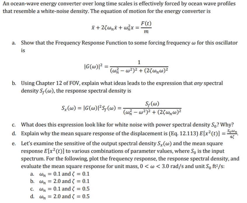 An ocean-wave energy converter over long time scales is effectively forced by ocean wave profiles
that resemble a white-noise density. The equation of motion for the energy converter is
F(t
£4 ant + ofr =D )
m
a. Show that the Frequency Response Function to some forcing frequency w for this oscillator
is
1
10) | Cl E—
16@F = Gor + @ana?
b. Using Chapter 12 of FOV, explain what ideas leads to the expression that any spectral
density S;(w), the response spectral density is
Sw)
5:(@) = 16) 2S (@) = ———r——
(©) = 16(w) 2S; (w) =a) + @oa?
c. What does this expression look like for white noise with power spectral density S,? Why?
d. Explain why the mean square response of the displacement is (Eq. 12.113) E[x?(t)] = a
e. Let's examine the sensitive of the output spectral density S, (w) and the mean square
response E[x?(t)] to various combinations of parameter values, where S, is the input
spectrum. For the following, plot the frequency response, the response spectral density, and
evaluate the mean square response for unit mass, 0 < < 3.0 rad/s and unit S ft/s:
a. w,=0land{=0.1
b. w,=20and{=01
¢ wp,=01and{=05
d w,=20and{=05