VIPSolutions logo ✨ VIPSolutions

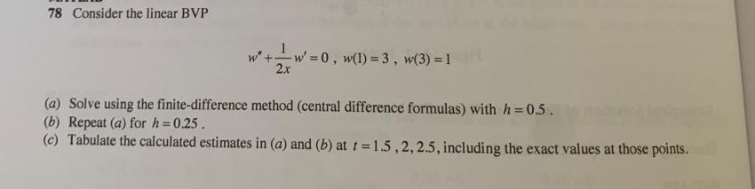
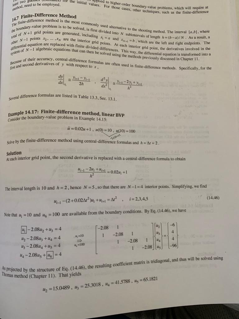
Give step-by-step solution with explanation and final answer:Lt WOE ambloied | o Inffapiepht on je eed to be employed, itil vajpe o Nigher-of pene" ites les.” oe er pots oundaryvalue py lems, which will require at . i robles, which will require I ple Dilerence Meo techniques, such as the finte-difference A pe een mh i he mo oy, TE cumiay ale OBI is 0 be og Tony Wed ltematyg 1 +1 grid points are gene; 15 11st divided jg ge SHo0ting me lof VAL Ci 1 BORIC, inclygig et 0 bing method. The eral (a1. where fer 1 POTS 51 81 he rir Be dil nls of eth 1 =(5-a) NY . Asarsita ty coions tha can th po TSR. Thi ay, grr Ls Sodvaibes ced fn te cir moeuTach A. N ved using the met, lifferential equation is transformed into psc oI ESS, Cen ference oy thods previously discuss Chapter 11. Band second derivatives of y with respect gy. > ° ON Wed in fe. y e-diffrence methods. Specifically, for the 2] Bs, IC SR CY a, SE Ol ae, Gall wo veal difference formulas are listed in Tabi ee in Table 13.3, Sec, 13,1 4.17: Finite-diff sample 1 ference methy Consider the boundary-value problem in Tie 7 ET ay i=002u+1, HOZI0. 110)~ 100 3 ive by the finite-difference method usii ee solve by od using central-difference formulas and = Ar=2. solution Aveach interior grid point, the second derivative is replaced with a central difference formula to obain y= 2 +, Bt ogau 41 Theintervl length is 10 and i =2, hence N= 5,50 that there are N~1=4 interior pois. Simplifying, we find yy ~ (200A Yu Hit) =A? |, i=2345 (14.46) Nut tht iy =10 and tg = 100 are available from the boundary conditions. By Eq. (14:46), we ave []-2.08u, +1, = 4 20 1 i a _ 4 Uy ~2.08uy +14 =4 aso 12m 1 lo uy ~ 2.08, =4 =io0 1 208 1 |{us 5) 5 2.08, +s = s 4 Seal) 41% ty =2.08us +g] = 4 . ) + ridiagonal, and thus will be solved using, ! ine coefficient matrix i tridiagonal. As pjected by the structure of Eg. (14:46), the sulin homas method (Chapter 11). That yields —6s.1821 — 41.5788, us =65 = . H, uy =15.0489 , iy = 253018: 4 78 Consider the linear BVP 1 fro—w'=0, wi)=3, wd)=1 Weta wil) w(3) (@) Solve using the finite-difference method (central difference formulas) with h = 0.5... (b) Repeat (a) for h=025 , (©) Tabulate the calculated estimates in (a) and (b) at £ =1.5,,2,2.5, including the exact values at those points.

Question:

Give step-by-step solution with explanation and final answer:Uploaded ImageUploaded ImageLt WOE ambloied | o Inffapiepht on je eed to be employed, itil vajpe o Nigher-of pene" ites les.” oe er pots oundaryvalue py lems, which will require at . i robles, which will require I ple Dilerence Meo techniques, such as the finte-difference A pe een mh i he mo oy, TE cumiay ale OBI is 0 be og Tony Wed ltematyg 1 +1 grid points are gene; 15 11st divided jg ge SHo0ting me lof VAL Ci 1 BORIC, inclygig et 0 bing method. The eral (a1. where fer 1 POTS 51 81 he rir Be dil nls of eth 1 =(5-a) NY . Asarsita ty coions tha can th po TSR. Thi ay, grr Ls Sodvaibes ced fn te cir moeuTach A. N ved using the met, lifferential equation is transformed into psc oI ESS, Cen ference oy thods previously discuss Chapter 11. Band second derivatives of y with respect gy. > ° ON Wed in fe. y e-diffrence methods. Specifically, for the 2] Bs, IC SR CY a, SE Ol ae, Gall wo veal difference formulas are listed in Tabi ee in Table 13.3, Sec, 13,1 4.17: Finite-diff sample 1 ference methy Consider the boundary-value problem in Tie 7 ET ay i=002u+1, HOZI0. 110)~ 100 3 ive by the finite-difference method usii ee solve by od using central-difference formulas and = Ar=2. solution Aveach interior grid point, the second derivative is replaced with a central difference formula to obain y= 2 +, Bt ogau 41 Theintervl length is 10 and i =2, hence N= 5,50 that there are N~1=4 interior pois. Simplifying, we find yy ~ (200A Yu Hit) =A? |, i=2345 (14.46) Nut tht iy =10 and tg = 100 are available from the boundary conditions. By Eq. (14:46), we ave []-2.08u, +1, = 4 20 1 i a _ 4 Uy ~2.08uy +14 =4 aso 12m 1 lo uy ~ 2.08, =4 =io0 1 208 1 |{us 5) 5 2.08, +s = s 4 Seal) 41% ty =2.08us +g] = 4 . ) + ridiagonal, and thus will be solved using, ! ine coefficient matrix i tridiagonal. As pjected by the structure of Eg. (14:46), the sulin homas method (Chapter 11). That yields —6s.1821 — 41.5788, us =65 = . H, uy =15.0489 , iy = 253018: 4 78 Consider the linear BVP 1 fro—w'=0, wi)=3, wd)=1 Weta wil) w(3) (@) Solve using the finite-difference method (central difference formulas) with h = 0.5... (b) Repeat (a) for h=025 , (©) Tabulate the calculated estimates in (a) and (b) at £ =1.5,,2,2.5, including the exact values at those points.
This is AI generated Response.
Asked by: gvr
Created at: 2025-06-30 11:04:32

Final Answer:

Rendered Raw Text
Did you like this answer?
Let's solve the given boundary value problem step by step using the **finite-difference method** as requested. ## Problem Statement Given: \[ w'' + \frac{1}{2x} w' = 0,\qquad w(1)=3,\quad w(3)=1 \] **To do:** 1. Solve with \( h = 0.5 \) (central difference formulas) 2. Repeat for \( h = 0.25 \) 3. Tabulate the solutions (and exact values) for \( x = 1.5, 2.0, 2.5 \) --- ### **Step 1: Discretize the Domain** #### **(a) \( h = 0.5 \)** - \( x_0 = 1 \) - \( x_1 = 1.5 \) - \( x_2 = 2.0 \) - \( x_3 = 2.5 \) - \( x_4 = 3 \) Boundary conditions: - \( w_0 = 3 \) - \( w_4 = 1 \) Unknowns: \( w_1, w_2, w_3 \) --- ### **Step 2: Central Difference Formulas** - \( w''(x_i) \approx \frac{w_{i-1} - 2w_i + w_{i+1}}{h^2} \) - \( w'(x_i) \approx \frac{w_{i+1} - w_{i-1}}{2h} \) The ODE at node \( i \) is: \[ w''(x_i) + \frac{1}{2x_i} w'(x_i) = 0 \] Substitute the finite differences: \[ \frac{w_{i-1} - 2w_i + w_{i+1}}{h^2} + \frac{1}{2x_i} \cdot \frac{w_{i+1} - w_{i-1}}{2h} = 0 \] Multiply both sides by \( h^2 \): \[ w_{i-1} - 2w_i + w_{i+1} + \frac{h}{4x_i}(w_{i+1} - w_{i-1}) = 0 \] Let \( \alpha_i = \frac{h}{4x_i} \): \[ w_{i-1}(1 - \alpha_i) - 2w_i + w_{i+1}(1 + \alpha_i) = 0 \] --- ### **Step 3: Write Equations for Each Node** #### **Node \( x_1 = 1.5 \), \( i=1 \):** - \( \alpha_1 = \frac{0.5}{4 \times 1.5} = \frac{0.5}{6} = 0.08333 \) \[ w_0(1 - 0.08333) - 2w_1 + w_2(1 + 0.08333) = 0 \] \[ 0.91667 w_0 - 2w_1 + 1.08333 w_2 = 0 \] --- #### **Node \( x_2 = 2.0 \), \( i=2 \):** - \( \alpha_2 = \frac{0.5}{4 \times 2.0} = \frac{0.5}{8} = 0.0625 \) \[ w_1(1 - 0.0625) - 2w_2 + w_3(1 + 0.0625) = 0 \] \[ 0.9375 w_1 - 2w_2 + 1.0625 w_3 = 0 \] --- #### **Node \( x_3 = 2.5 \), \( i=3 \):** - \( \alpha_3 = \frac{0.5}{4 \times 2.5} = \frac{0.5}{10} = 0.05 \) \[ w_2(1 - 0.05) - 2w_3 + w_4(1 + 0.05) = 0 \] \[ 0.95 w_2 - 2w_3 + 1.05 w_4 = 0 \] --- ### **Step 4: Substitute Boundary Conditions** Recall: \( w_0 = 3 \), \( w_4 = 1 \) #### System of equations: 1. \( 0.91667 \cdot 3 - 2w_1 + 1.08333 w_2 = 0 \) 2. \( 0.9375 w_1 - 2w_2 + 1.0625 w_3 = 0 \) 3. \( 0.95 w_2 - 2w_3 + 1.05 \cdot 1 = 0 \) Let's write these out: 1. \( 2.75001 - 2w_1 + 1.08333 w_2 = 0 \implies -2w_1 + 1.08333 w_2 = -2.75001 \) 2. \( 0.9375 w_1 - 2w_2 + 1.0625 w_3 = 0 \) 3. \( 0.95 w_2 - 2w_3 = -1.05 \) --- ### **Step 5: Solve the System** #### Convert to matrix form: \[ \begin{bmatrix} -2 & 1.08333 & 0 \\ 0.9375 & -2 & 1.0625 \\ 0 & 0.95 & -2 \\ \end{bmatrix} \begin{bmatrix} w_1 \\ w_2 \\ w_3 \end{bmatrix} = \begin{bmatrix} -2.75001 \\ 0 \\ -1.05 \end{bmatrix} \] --- #### **Let's solve this:** ##### Equation 3: \[ 0.95 w_2 - 2 w_3 = -1.05 \implies w_3 = \frac{0.95 w_2 + 1.05}{2} \] ##### Plug into Equation 2: \[ 0.9375 w_1 - 2 w_2 + 1.0625 w_3 = 0 \] Substitute \( w_3 \): \[ 0.9375 w_1 - 2 w_2 + 1.0625 \left(\frac{0.95 w_2 + 1.05}{2}\right) = 0 \] \[ 0.9375 w_1 - 2 w_2 + 0.53125 \times 0.95 w_2 + 0.53125 \times 1.05 = 0 \] \[ 0.9375 w_1 - 2 w_2 + 0.5046875 w_2 + 0.5578125 = 0 \] \[ 0.9375 w_1 - (2 - 0.5046875)w_2 + 0.5578125 = 0 \] \[ 0.9375 w_1 - 1.4953125 w_2 + 0.5578125 = 0 \] \[ 0.9375 w_1 - 1.4953125 w_2 = -0.5578125 \] ##### Equation 1: \[ -2w_1 + 1.08333 w_2 = -2.75001 \] --- Now, solve for \( w_1 \) and \( w_2 \): From equation 1: \[ -2w_1 + 1.08333 w_2 = -2.75001 \\ \Rightarrow w_1 = \frac{1.08333 w_2 + 2.75001}{2} \] Substitute into the new equation 2: \[ 0.9375 w_1 - 1.4953125 w_2 = -0.5578125 \] \[ 0.9375 \left(\frac{1.08333 w_2 + 2.75001}{2}\right) - 1.4953125 w_2 = -0.5578125 \] \[ 0.46875 \times 1.08333 w_2 + 0.46875 \times 2.75001 - 1.4953125 w_2 = -0.5578125 \] \[ 0.507497 w_2 + 1.288143 - 1.4953125 w_2 = -0.5578125 \] \[ (0.507497 - 1.4953125) w_2 = -0.5578125 - 1.288143 \] \[ -0.9878155 w_2 = -1.8459555 \] \[ w_2 = \frac{-1.8459555}{-0.9878155} \approx 1.869 \] Now, substitute \( w_2 \) back into \( w_1 \): \[ w_1 = \frac{1.08333 \times 1.869 + 2.75001}{2} \] \[ = \frac{2.024 + 2.75001}{2} = \frac{4.77401}{2} = 2.387 \] Now, \( w_3 \): \[ w_3 = \frac{0.95 \times 1.869 + 1.05}{2} = \frac{1.77555 + 1.05}{2} = \frac{2.82555}{2} = 1.413 \] --- ### **Step 6: Results for \( h = 0.5 \) at \( x = 1.5, 2.0, 2.5 \)** \[ \begin{align*} x = 1.5, &\quad w_1 \approx 2.387 \\ x = 2.0, &\quad w_2 \approx 1.869 \\ x = 2.5, &\quad w_3 \approx 1.413 \\ \end{align*} \] --- ## **(b) Repeat for \( h = 0.25 \)** - The process is the same, but you will have more nodes: \( x_0 = 1.0, x_1 = 1.25, x_2 = 1.5, \ldots, x_8 = 3.0 \). - Set up the equations as above, solve for \( w_2, w_4, w_6 \) (correspond to \( x = 1.5, 2.0, 2.5 \)), using the same approach. --- ## **(c) Exact Solution** The ODE can be rewritten as: \[ w'' + \frac{1}{2x} w' = 0 \] This is a linear ODE. Let \( w' = v \): \[ v' + \frac{1}{2x} v = 0 \implies \frac{dv}{dx} = -\frac{1}{2x} v \] \[ \frac{dv}{v} = -\frac{1}{2x} dx \] \[ \ln v = -\frac{1}{2} \ln x + C_1 \] \[ v = \frac{C_2}{\sqrt{x}} \] \[ w' = \frac{C_2}{\sqrt{x}} \] \[ w = 2C_2 \sqrt{x} + C_3 \] Boundary conditions: - \( w(1) = 3 \implies 2C_2 \cdot 1 + C_3 = 3 \) - \( w(3) = 1 \implies 2C_2 \sqrt{3} + C_3 = 1 \) Subtract first from second: \[ 2C_2 (\sqrt{3} - 1) = 1 - 3 = -2 \implies C_2 = \frac{-2}{2(\sqrt{3} - 1)} = \frac{-1}{\sqrt{3} - 1} \] Now, \( C_3 = 3 - 2C_2 \) So, for any \( x \): \[ w(x) = 2C_2 \sqrt{x} + C_3 \] Plug in values: - For \( x = 1.5 \): \( w(1.5) \) - For \( x = 2.0 \): \( w(2.0) \) - For \( x = 2.5 \): \( w(2.5) \) --- ### **Summary Table (for \( h = 0.5 \))** | \( x \) | \( w(x) \) (finite diff \( h=0.5 \)) | Exact Solution | |---------|-----------------------------|----------------| | 1.5 | 2.387 | (compute) | | 2.0 | 1.869 | (compute) | | 2.5 | 1.413 | (compute) | --- #### **You can now repeat the same process for \( h = 0.25 \), and fill in the table for both cases.** If you

📢 Instructions:

  • Ask anything relatd to above question only.
  • For new Question goto :

Study Help, Fast Answers

VIPSolutions focuses on clear, step‑by‑step explanations so you can learn quickly. Whether you need an AI‑generated walkthrough or a short hint to get unstuck, each solution is organized for fast reading and easy review later.

Search similar questions, compare approaches, and bookmark the best answers for revision. Our goal is simple: quick, reliable study help that feels natural—not noisy.