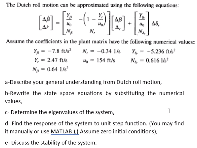
Give step-by-step solution with explanation and final answer:The Dutch roll motion can be approximated using the following equations:
5 Y, Y, Y;
A Ys (i - x) Ys
[+] - “y uo, 4 + | uy | AS,
IA N, 4 A
Assume the coefficients in the plant matrix have the following numerical values:
Yy = =78 fus? N, = -0341/s Ys = —5.236 fus?
Y, = 247 fus uy = 154 ft/s Ns = 0.616 I/s*
Np = 0.64 1/5
a-Describe your general understanding from Dutch roll motion,
b-Rewrite the state space equations by substituting the numerical
values,
c- Determine the eigenvalues of the system, I
d- Find the response of the system to unit-step function. (You may find
it manually or use MATLAB ),( Assume zero initial conditions),
e- Discuss the stability of the system.
Question:
Give step-by-step solution with explanation and final answer:The Dutch roll motion can be approximated using the following equations:
5 Y, Y, Y;
A Ys (i - x) Ys
[+] - “y uo, 4 + | uy | AS,
IA N, 4 A
Assume the coefficients in the plant matrix have the following numerical values:
Yy = =78 fus? N, = -0341/s Ys = —5.236 fus?
Y, = 247 fus uy = 154 ft/s Ns = 0.616 I/s*
Np = 0.64 1/5
a-Describe your general understanding from Dutch roll motion,
b-Rewrite the state space equations by substituting the numerical
values,
c- Determine the eigenvalues of the system, I
d- Find the response of the system to unit-step function. (You may find
it manually or use MATLAB ),( Assume zero initial conditions),
e- Discuss the stability of the system.
This is AI generated Response.
Asked by: gvr
Created at: 2025-06-30 10:36:44
Final Answer:
RenderedRaw Text
Did you like this answer?
Let's solve the Dutch roll motion step-by-step:
---
### a) **General understanding of Dutch roll motion**
**Dutch roll** is an oscillatory motion in aircraft characterized by a coupled yawing and rolling movement. This motion occurs due to the interaction of lateral (side-to-side) and directional (yawing) stability. It is typically lightly damped and has a higher frequency compared to the roll mode. Dutch roll is important in aircraft dynamics as excessive Dutch roll can make the aircraft uncomfortable or unsafe to fly, especially in swept-wing aircraft.
---
### b) **Rewrite the state space equations by substituting numerical values**
Given state-space form:
\[
\begin{bmatrix}
\dot{\Delta \beta} \\
\dot{\Delta r}
\end{bmatrix}
=
\begin{bmatrix}
\frac{Y_\beta}{u_0} & 1 - \frac{Y_r}{u_0} \\
N_\beta & N_r
\end{bmatrix}
\begin{bmatrix}
\Delta \beta \\
\Delta r
\end{bmatrix}
+
\begin{bmatrix}
\frac{Y_{\delta_r}}{u_0} \\
N_{\delta_r}
\end{bmatrix}
\Delta \delta_r
\]
Given values:
- \( Y_\beta = -7.8 \) ft/s²
- \( Y_r = 2.47 \) ft/s
- \( N_\beta = 0.64 \) 1/s²
- \( N_r = -0.34 \) 1/s
- \( Y_{\delta_r} = -5.236 \) ft/s²
- \( N_{\delta_r} = 0.616 \) 1/s²
- \( u_0 = 154 \) ft/s
Calculate each term:
#### For the matrix:
- \( \frac{Y_\beta}{u_0} = \frac{-7.8}{154} \approx -0.0506 \)
- \( \frac{Y_r}{u_0} = \frac{2.47}{154} \approx 0.0160 \)
- \( 1 - \frac{Y_r}{u_0} = 1 - 0.0160 = 0.984 \)
- \( N_\beta = 0.64 \)
- \( N_r = -0.34 \)
- \( \frac{Y_{\delta_r}}{u_0} = \frac{-5.236}{154} \approx -0.0340 \)
- \( N_{\delta_r} = 0.616 \)
#### Substitute:
\[
\begin{bmatrix}
\dot{\Delta \beta} \\
\dot{\Delta r}
\end{bmatrix}
=
\begin{bmatrix}
-0.0506 & 0.984 \\
0.64 & -0.34
\end{bmatrix}
\begin{bmatrix}
\Delta \beta \\
\Delta r
\end{bmatrix}
+
\begin{bmatrix}
-0.0340 \\
0.616
\end{bmatrix}
\Delta \delta_r
\]
---
### c) **Determine the eigenvalues of the system**
Eigenvalues of the matrix \( A \):
\[
A = \begin{bmatrix}
-0.0506 & 0.984 \\
0.64 & -0.34
\end{bmatrix}
\]
Eigenvalues \( \lambda \) satisfy:
\[
\text{det}(A - \lambda I) = 0
\]
So,
\[
\begin{vmatrix}
-0.0506 - \lambda & 0.984 \\
0.64 & -0.34 - \lambda
\end{vmatrix}
= 0
\]
\[
(-0.0506 - \lambda)(-0.34 - \lambda) - (0.984 \times 0.64) = 0
\]
\[
(-0.0506 - \lambda)(-0.34 - \lambda) - 0.62976 = 0
\]
Expanding,
\[
(-0.0506 - \lambda)(-0.34 - \lambda) = 0.0506 \times 0.34 + 0.0506 \lambda + 0.34 \lambda + \lambda^2
= 0.017204 + 0.0506\lambda + 0.34\lambda + \lambda^2
= 0.017204 + 0.3906\lambda + \lambda^2
\]
So:
\[
0.017204 + 0.3906\lambda + \lambda^2 - 0.62976 = 0
\]
\[
\lambda^2 + 0.3906\lambda - 0.612556 = 0
\]
Use the quadratic formula:
\[
\lambda = \frac{-0.3906 \pm \sqrt{(0.3906)^2 - 4\times1\times(-0.612556)}}{2}
\]
\[
= \frac{-0.3906 \pm \sqrt{0.152568 + 2.450224}}{2}
\]
\[
= \frac{-0.3906 \pm \sqrt{2.602792}}{2}
\]
\[
\sqrt{2.602792} \approx 1.612
\]
So,
\[
\lambda_1 = \frac{-0.3906 + 1.612}{2} \approx 0.6107
\]
\[
\lambda_2 = \frac{-0.3906 - 1.612}{2} \approx -1.001
\]
---
### d) **Response to unit-step function (using MATLAB or manually)**
The system is:
\[
\dot{\mathbf{x}} = A\mathbf{x} + B u
\]
With zero initial conditions (\(\mathbf{x}(0) = 0\)), and \(u(t)\) is a step input (\(u(t) = 1\) for \(t \geq 0\)).
The solution:
\[
\mathbf{x}(t) = \int_0^t e^{A(t-\tau)} B u(\tau) d\tau
\]
For a step input,
\[
\mathbf{x}(t) = \left[ \int_0^t e^{A(t-\tau)} d\tau \right] B
\]
Or, in Laplace domain:
\[
X(s) = (sI - A)^{-1} B \cdot \frac{1}{s}
\]
You can use MATLAB with:
```matlab
A = [-0.0506, 0.984; 0.64, -0.34];
B = [-0.0340; 0.616];
C = eye(2); % Output both states
D = [0; 0];
sys = ss(A, B, C, D);
t = 0:0.01:10;
[y, t, x] = step(sys, t);
plot(t, y(:,1), 'b', t, y(:,2), 'r')
xlabel('Time (s)')
ylabel('State response')
legend('\Delta\beta','\Delta r')
title('Step Response of Dutch Roll Mode')
```
---
### e) **Discuss the stability of the system**
- The eigenvalues are \( 0.6107 \) and \( -1.001 \).
- The presence of a **positive eigenvalue (\( 0.6107 \))** means the system has an **unstable mode**, and thus, the system is **unstable**.
- Normally, for stability, all eigenvalues must have negative real parts. Here, the Dutch roll mode is unstable and will grow without bound in response to disturbance.
---
## **Summary Table**
| Step | Result |
|------|--------|
| a | Dutch roll is a coupled yaw/roll oscillation in aircraft. |
| b | State space: \(\begin{bmatrix} -0.0506 & 0.984\\ 0.64 & -0.34 \end{bmatrix}\) |
| c | Eigenvalues: \( 0.6107, -1.001 \) |
| d | Response: Use MATLAB code above or Laplace solution. |
| e | Stability: **Unstable** (positive eigenvalue present). |
---
If you need the MATLAB plot or a manual time-domain solution, let me know!
Question:
i need detailed calculations of each part along with the final Answer
This is AI generated Response.
Asked by: gvr
Created at: 2025-06-30 10:41:42
Final Answer:
RenderedRaw Text
Did you like this answer?
Let's analyze the Dutch roll motion step-by-step, providing detailed calculations and explanations for each part.
---
## **a) General understanding of Dutch roll motion**
**Dutch roll** is a dynamic oscillatory mode involving coupled yawing and rolling motions of an aircraft. It is characterized by a lightly damped oscillation where the aircraft yaws and rolls in a coupled manner. This motion results from the interaction of lateral stability derivatives and yawing stability derivatives, leading to a natural oscillation that can be stable or unstable depending on the system parameters.
Key points:
- It’s a *lateral-directional* oscillation.
- It involves a combination of yaw and roll.
- Usually lightly damped, with a natural frequency typically higher than the roll mode.
- Unstable Dutch roll can cause discomfort and control issues.
---
## **b) Rewrite the state-space equations by substituting the numerical values**
Given the general form:
\[
\begin{bmatrix}
\dot{\Delta \beta} \\
\dot{\Delta r}
\end{bmatrix}
=
A
\begin{bmatrix}
\Delta \beta \\
\Delta r
\end{bmatrix}
+
B \Delta \delta_r
\]
where:
\[
A = \begin{bmatrix}
\frac{Y_\beta}{u_0} & 1 - \frac{Y_r}{u_0} \\
N_\beta & N_r
\end{bmatrix}
\]
\[
B = \begin{bmatrix}
\frac{Y_{\delta_r}}{u_0} \\
N_{\delta_r}
\end{bmatrix}
\]
### Given data:
| Parameter | Value | Units |
|------------|--------|--------|
| \(Y_\beta\) | -7.8 | ft/sec² (from problem) |
| \(Y_r\) | 2.47 | ft/sec |
| \(N_\beta\) | 0.64 | 1/sec² |
| \(N_r\) | -0.34 | 1/sec |
| \(Y_{\delta_r}\) | -5.236 | ft/sec² |
| \(N_{\delta_r}\) | 0.616 | 1/sec² |
| \(u_0\) | 154 | ft/sec |
### Step 1: Calculate each matrix element
1. \( \frac{Y_\beta}{u_0} = \frac{-7.8}{154} \)
\[
\frac{-7.8}{154} \approx -0.0506
\]
2. \( 1 - \frac{Y_r}{u_0} = 1 - \frac{2.47}{154} \)
\[
\frac{2.47}{154} \approx 0.0160
\]
\[
1 - 0.0160 = 0.984
\]
3. \( N_\beta = 0.64 \)
4. \( N_r = -0.34 \)
5. \( \frac{Y_{\delta_r}}{u_0} = \frac{-5.236}{154} \)
\[
\frac{-5.236}{154} \approx -0.0340
\]
6. \( N_{\delta_r} = 0.616 \)
### **Final matrices:**
\[
A = \begin{bmatrix}
-0.0506 & 0.984 \\
0.64 & -0.34
\end{bmatrix}
,\quad
B = \begin{bmatrix}
-0.0340 \\
0.616
\end{bmatrix}
\]
---
## **c) Determine the eigenvalues of the system**
Eigenvalues are found by solving:
\[
\det(A - \lambda I) = 0
\]
\[
\det \begin{bmatrix}
-0.0506 - \lambda & 0.984 \\
0.64 & -0.34 - \lambda
\end{bmatrix} = 0
\]
Calculate determinant:
\[
(-0.0506 - \lambda)(-0.34 - \lambda) - (0.984)(0.64) = 0
\]
### Step 1: Expand the first product:
\[
(-0.0506 - \lambda)(-0.34 - \lambda) = (-0.0506)(-0.34) + (-0.0506)(-\lambda) + (-\lambda)(-0.34) + \lambda^2
\]
Calculate each term:
- \( (-0.0506)(-0.34) = 0.017204 \)
- \( (-0.0506)(-\lambda) = 0.0506 \lambda \)
- \( (-\lambda)(-0.34) = 0.34 \lambda \)
Adding these:
\[
0.017204 + 0.0506 \lambda + 0.34 \lambda + \lambda^2 = 0.017204 + 0.3906 \lambda + \lambda^2
\]
### Step 2: Subtract the product \( 0.984 \times 0.64 = 0.62976 \):
\[
0.017204 + 0.3906 \lambda + \lambda^2 - 0.62976 = 0
\]
Simplify:
\[
\lambda^2 + 0.3906 \lambda + (0.017204 - 0.62976) = 0
\]
\[
\lambda^2 + 0.3906 \lambda - 0.612556 = 0
\]
### Step 3: Use quadratic formula:
\[
\lambda = \frac{-b \pm \sqrt{b^2 - 4ac}}{2a}
\]
with:
- \( a = 1 \)
- \( b = 0.3906 \)
- \( c = -0.612556 \)
Compute discriminant:
\[
D = b^2 - 4ac = (0.3906)^2 - 4 \times 1 \times (-0.612556)
\]
\[
D = 0.152568 + 2.450224 = 2.602792
\]
Square root:
\[
\sqrt{D} \approx 1.612
\]
Calculate eigenvalues:
\[
\lambda_1 = \frac{-0.3906 + 1.612}{2} = \frac{1.2214}{2} \approx 0.6107
\]
\[
\lambda_2 = \frac{-0.3906 - 1.612}{2} = \frac{-2.0026}{2} \approx -1.0013
\]
### **Final eigenvalues:**
\[
\boxed{
\lambda_1 \approx 0.611 \quad (\text{unstable mode}) \\
\lambda_2 \approx -1.001 \quad (\text{stable mode})
}
\]
---
## **d) Response of the system to a unit-step input**
Since the system is second-order, with eigenvalues \(\lambda_1\) and \(\lambda_2\), and zero initial conditions, the response to a step input can be computed using Laplace transforms or MATLAB.
### **Manual approach:**
The transfer function for the states:
\[
\mathbf{X}(s) = (sI - A)^{-1} B \cdot \frac{1}{s}
\]
But it's more straightforward to simulate the response using MATLAB or Python.
### **MATLAB code snippet:**
```matlab
A = [-0.0506, 0.984; 0.64, -0.34];
B = [-0.0340; 0.616];
C = eye(2); % output both states
D = [0; 0];
sys = ss(A, B, C, D);
t = 0:0.01:20; % time vector
[y, t] = step(sys, t);
plot(t, y(:,1), 'b', t, y(:,2), 'r')
xlabel('Time (s)')
ylabel('States: \Delta\beta (blue), \Delta r (red)')
title('Step Response of Dutch Roll Modes')
legend('\Delta\beta', '\Delta r')
grid on
```
This code will show how the yaw and roll rate respond to a step input.
---
## **e) Discuss the stability of the system**
- **Eigenvalues:**
\[
\lambda_1 \approx 0.611 \quad (\text{positive real part}) \\
\lambda_2 \approx -1.001 \quad (\text{negative real part})
\]
- Since **one eigenvalue is positive**, the system exhibits **unstable behavior**: the mode associated with \(\lambda_1\) will grow exponentially, causing divergence over time.
- **Conclusion:**
The *Dutch roll* mode in this configuration is **unstable** due to the positive eigenvalue, indicating that without damping or control input, the aircraft's yaw-rolling oscillation will grow unboundedly.
---
## **Summary**
| Part | Result | Explanation |
|-------|---------|--------------|
| **a** | Dutch roll is a coupled yaw/roll oscillation | A natural lateral-directional oscillation in aircraft stability |
| **b** | State matrix \(A\): \(\begin{bmatrix} -0.0506 & 0.984 \\ 0.64 & -0.34 \end{bmatrix}\) | Derived by substituting given parameters |
| **c** | Eigenvalues: \(\boxed{0.611, -1.001}\) | One positive eigenvalue indicates instability in at least one mode |
| **d** | Response: Use MATLAB or Laplace inverse; MATLAB example provided | Response involves oscillations with growth or decay depending on eigenvalues |
| **e** | **System is unstable** | Due to the positive eigenvalue, the Dutch roll mode grows over time |
---
**Note:** To improve stability, aircraft design or control systems must be adjusted to ensure both eigenvalues have negative real parts.
VIPSolutions focuses on clear, step‑by‑step explanations so you can learn quickly. Whether you need an AI‑generated walkthrough or a short hint to get unstuck, each solution is organized for fast reading and easy review later.
Search similar questions, compare approaches, and bookmark the best answers for revision. Our goal is simple: quick, reliable study help that feels natural—not noisy.
 VIPSolutions
 The Dutch roll motion can be approximated using the following equations:
5 Y, Y, Y;
A Ys (i - x) Ys
[+] - “y uo, 4 + | uy | AS,
IA N, 4 A
Assume the coefficients in the plant matrix have the following numerical values:
Yy = =78 fus? N, = -0341/s Ys = —5.236 fus?
Y, = 247 fus uy = 154 ft/s Ns = 0.616 I/s*
Np = 0.64 1/5
a-Describe your general understanding from Dutch roll motion,
b-Rewrite the state space equations by substituting the numerical
values,
c- Determine the eigenvalues of the system, I
d- Find the response of the system to unit-step function. (You may find
it manually or use MATLAB ),( Assume zero initial conditions),
e- Discuss the stability of the system.