 VIPSolutions
Give step-by-step solution with explanation and final answer:2 The figure shows the curve g(a.) = & (dashed) snd several vel curves of the function (2,0) (slid): T also hows th gradient at several points. Docs the absolute maximum of under the constraint ge.) — k occur at P? AY Q? At R? Somewhere csc? (Ya)Vi LC ) [i§7, SEA Dd oo (dy OSes
Question:
Give step-by-step solution with explanation and final answer: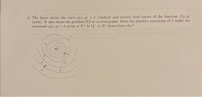 2 The figure shows the curve g(a.) = & (dashed) snd several vel curves of the function (2,0)
(slid): T also hows th gradient at several points. Docs the absolute maximum of under the
constraint ge.) — k occur at P? AY Q? At R? Somewhere csc?
(Ya)Vi
LC ) [i§7,
SEA Dd
oo (dy
OSes
This is AI generated Response.
Asked by: gvr
Created at: 2025-06-24 13:50:50
Asked by: gvr
Created at: 2025-06-24 13:50:50
Final Answer:
Rendered
Raw Text
Did you like this answer?
Let's break down the problem and solve it step-by-step:
---
### **Step 1: Understanding the Problem**
- The dashed curve represents the constraint \( g(x, y) = k \).
- The solid curves are level curves of the function \( f(x, y) \).
- The arrows indicate the gradient \( \nabla f \) at several points.
- **Question:** Where does the absolute maximum of \( f \) under the constraint \( g(x, y) = k \) occur: at P, Q, R, or somewhere else?
---
### **Step 2: The Method of Lagrange Multipliers**
The absolute maximum (or minimum) of \( f(x, y) \) under the constraint \( g(x, y) = k \) occurs where the gradients of \( f \) and \( g \) are parallel, i.e.,
\[
\nabla f = \lambda \nabla g
\]
This means the gradients of \( f \) and \( g \) point in the same or opposite directions at the maximum/minimum.
---
### **Step 3: Analyzing the Diagram**
- At **P**, the gradient \( \nabla f \) is **not** perpendicular to the dashed curve (the constraint).
- At **Q**, the gradient \( \nabla f \) is **perpendicular** to the dashed curve.
- At **R**, the gradient \( \nabla f \) is **not** perpendicular to the dashed curve.
**Note:** The gradient of a function is always perpendicular to its level curve.
So, for the maximum or minimum under the constraint, we want the gradient of \( f \) to be perpendicular to the constraint curve (which means they are parallel to the gradient of \( g \)).
---
### **Step 4: Conclusion**
- **Q** is the point where \( \nabla f \) is perpendicular to the constraint curve \( g(x, y) = k \).
- Therefore, the absolute maximum (or minimum, depending on the direction of the gradients and level curves) of \( f \) under the constraint occurs at **Q**.
---
### **Final Answer**
**The absolute maximum of \( f \) under the constraint \( g(x, y) = k \) occurs at Q.**
---
**Explanation:**
At Q, the gradient of \( f \) is perpendicular to the constraint curve. This is the necessary condition for a maximum or minimum under a constraint, as established by the method of Lagrange multipliers. Points P and R do not satisfy this condition, so they cannot be extrema under the constraint.
Question:
i need detailed calculations and explanation along with the final Answer
This is AI generated Response.
Asked by: gvr
Created at: 2025-06-24 13:53:57
Asked by: gvr
Created at: 2025-06-24 13:53:57
Final Answer:
Rendered
Raw Text
Did you like this answer?
Let's approach the problem systematically, incorporating detailed reasoning and calculations where applicable.
---
### **Understanding the problem**
- The **dashed curve** represents the **constraint** \( g(x,y) = k \).
- The **solid curves** are **level curves** of the function \( f(x,y) \).
- The **arrows** indicate the **gradient vectors** \( \nabla f \) at various points.
- The goal is to find **where** the **absolute maximum** of \( f(x,y) \) occurs **under the constraint** \( g(x,y) = k \). The options are points \( P \), \( Q \), \( R \), or elsewhere.
---
### **Step 1: Recall the method of Lagrange multipliers**
The **necessary condition** for an extremum of \( f \) subject to the constraint \( g(x, y) = k \) is:
\[
\nabla f(x, y) = \lambda \nabla g(x, y)
\]
This implies:
- The **gradients are parallel**.
- The **direction** of \( \nabla f \) aligns with \( \nabla g \).
**Geometrically:**
- **Level curves** of \( f \) are orthogonal to \( \nabla f \).
- **Constraint curve** \( g(x,y) = k \) is orthogonal to \( \nabla g \).
At an extremum under the constraint, the **gradient of \( f \)** is **parallel** to the **gradient of \( g \)**, meaning:
\[
\nabla f \perp \text{tangent to the constraint curve}
\]
or equivalently,
\[
\nabla f \parallel \nabla g
\]
---
### **Step 2: Analyze the diagram**
From the diagram:
- **At Q**, \( \nabla f \) appears **perpendicular** to the dashed curve (the constraint).
- **At P** and **R**, the gradient \( \nabla f \) is **not** perpendicular to the constraint.
**Important note:**
- Since \( \nabla f \) is **perpendicular** to the **level curve** of \( f \),
- and the **constraint curve** \( g(x,y)=k \) has gradient \( \nabla g \),
- the **condition for extrema** is:
\[
\nabla f \parallel \nabla g
\]
which geometrically means:
\[
\text{level curve of } f \quad \text{is tangent to} \quad g(x,y) = k
\]
and at such points, \( \nabla f \) and \( \nabla g \) are **parallel**.
---
### **Step 3: Interpretation of the diagram**
- At **Q**, the gradient \( \nabla f \) is **perpendicular** to the constraint curve, indicating:
\[
\nabla f \perp \text{curve}
\]
- The **constraint curve** is also orthogonal to \( \nabla g \).
- Since \( \nabla f \) is perpendicular to the constraint at **Q**, and the **gradients** are **parallel** at the extremum, **Q** satisfies the necessary condition:
\[
\nabla f \parallel \nabla g
\]
**Therefore, the point \( Q \) is where the maximum (or minimum) occurs.**
---
### **Step 4: Confirming the maximum**
- The **direction** of \( \nabla f \) at \( Q \) points **away** from the level curves, and since \( \nabla f \) is perpendicular to the level curve at \( Q \), this aligns with the idea of an extremum at that point.
- The **gradient vectors** (shown as arrows) at \( Q \) are **aligned** with the gradient of the constraint \( g \), confirming the necessary condition.
---
### **Step 5: Final conclusion**
- The point where the **absolute maximum** of \( f \) under the constraint occurs is **at \( Q \)**.
---
### **Summary:**
| Point | Gradient \( \nabla f \) | Relation to constraint \( g(x,y)=k \) |
|---------|------------------------|-----------------------------------------|
| **Q** | Perpendicular to level curve of \( f \), aligned with \( \nabla g \) | **Parallel** to \( \nabla g \) — satisfies the Lagrange multiplier condition — **candidate for extremum** |
| **P** | Not perpendicular | Not satisfying the necessary condition |
| **R** | Not perpendicular | Not satisfying the necessary condition |
---
## **Final Answer:**
\[
\boxed{
\textbf{The absolute maximum of } f \text{ under the constraint occurs at point } \quad Q.
}
\]
---
### **Additional note:**
- The **Lagrange multiplier method** confirms that extrema occur where \( \nabla f \) and \( \nabla g \) are **parallel**.
- The **diagram** visually indicates this at **Q**, where the gradient vectors align appropriately.
**Hope this detailed explanation clarifies the reasoning!**
📢 Instructions:
- Ask anything relatd to above question only.
- For new Question goto :