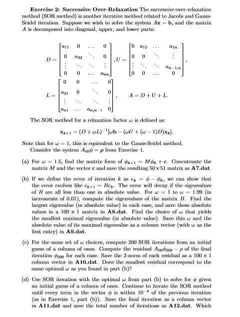
Let's break down and solve each part step by step. We’ll assume you have the matrix **A** and vector **b** from the previous exercise, and focus on the SOR method as described. --- ### **Part (a): Matrix Form of φ_k+1** Given: - **ω = 1.5** - SOR update formula: \[ \mathbf{x}_{k+1} = (D + \omega L)^{-1} [\omega \mathbf{b} - (\omega U + (\omega - 1) D)\mathbf{x}_k] \] where \(A = D + U + L\). Let’s write this as: \[ \phi_{k+1} = M \phi_k + c \] where: - \(M = (D + \omega L)^{-1} [-(\omega U + (\omega - 1) D)]\) - \(c = (D + \omega L)^{-1} [\omega \mathbf{b}]\) **To construct the 50x51 matrix:** - Concatenate \(M\) (which is 50x50) and \(c\) (which is 50x1) as columns to form a 50x51 matrix. **Save as:** `A7.dat` **Python-like pseudocode:** ```python import numpy as np # Assuming A and b are already defined (A is 50x50, b is 50x1) n = A.shape[0] omega = 1.5 D = np.diag(np.diag(A)) L = np.tril(A, k=-1) U = np.triu(A, k=1) M = np.linalg.inv(D + omega * L) @ (-(omega * U + (omega - 1) * D)) c = np.linalg.inv(D + omega * L) @ (omega * b) A7 = np.column_stack((M, c)) np.savetxt('A7.dat', A7) ``` --- ### **Part (b): Eigenvalues of B for Different ω** **Matrix B:** \[ B = (D + \omega L)^{-1} (\omega U + (\omega - 1) D) \] **Steps:** 1. For ω from 1 to 1.99 in steps of 0.01: - Compute B for each ω. - Compute all eigenvalues of B. - Record the largest eigenvalue in absolute value (spectral radius). 2. Save the 100 x 1 matrix of largest eigenvalues as `A8.dat`. 3. Find ω that yields the smallest spectral radius. Save ω and the smallest value as `A9.dat`. **Python-like pseudocode:** ```python omegas = np.arange(1.00, 2.00, 0.01) spectral_radii = [] for omega in omegas: B = np.linalg.inv(D + omega * L) @ (omega * U + (omega - 1) * D) eigvals = np.linalg.eigvals(B) spectral_radii.append(np.max(np.abs(eigvals))) A8 = np.array(spectral_radii).reshape(-1, 1) np.savetxt('A8.dat', A8) min_idx = np.argmin(A8) best_omega = omegas[min_idx] min_radius = A8[min_idx, 0] np.savetxt('A9.dat', np.array([best_omega, min_radius])) ``` --- ### **Part (c): SOR Residuals for Each ω** 1. For each ω, perform 200 SOR iterations starting from an initial guess (e.g., zeros). 2. At each ω, compute the residual after 200 iterations: \( r = A\phi_{200} - b \) 3. Compute the 2-norm of each residual and save as a 100x1 column vector in `A10.dat`. **Python-like pseudocode:** ```python A10 = [] for omega in omegas: x = np.zeros((n, 1)) for k in range(200): for i in range(n): sum1 = np.dot(A[i, :i], x[:i]) sum2 = np.dot(A[i, i+1:], x[i+1:]) x[i] = (1 - omega) * x[i] + (omega / A[i, i]) * (b[i] - sum1 - sum2) residual = A @ x - b A10.append(np.linalg.norm(residual)) A10 = np.array(A10).reshape(-1, 1) np.savetxt('A10.dat', A10) ``` --- ### **Part (d): SOR Until Convergence for Best ω** 1. Use the ω value from (b) that gave the smallest spectral radius. 2. Start from an initial guess (e.g., zeros). 3. Iterate SOR until the relative error in the vector φ is less than \(10^{-4}\) of the previous iteration. 4. Save the final solution as a column vector in `A11.dat`. 5. Save the total number of iterations in `A12.dat`. **Python-like pseudocode:** ```python omega = best_omega x = np.zeros((n, 1)) tol = 1e-4 max_iter = 10000 count = 0 while True: x_old = x.copy() for i in range(n): sum1 = np.dot(A[i, :i], x[:i]) sum2 = np.dot(A[i, i+1:], x[i+1:]) x[i] = (1 - omega) * x[i] + (omega / A[i, i]) * (b[i] - sum1 - sum2) count += 1 if np.linalg.norm(x - x_old) < tol * np.linalg.norm(x_old) or count >= max_iter: break np.savetxt('A11.dat', x) np.savetxt('A12.dat', np.array([count])) ``` --- ## **Summary of Outputs:** - **A7.dat:** 50x51 matrix concatenating M and c. - **A8.dat:** 100x1 column of spectral radii for ω = 1.00, ..., 1.99. - **A9.dat:** 2x1 vector: [optimal ω, min spectral radius]. - **A10.dat:** 100x1 column of 2-norm residuals for each ω after 200 iterations. - **A11.dat:** 50x1 solution vector for optimal ω. - **A12.dat:** Number of iterations to reach convergence for optimal ω. --- If you have your matrix **A** and vector **b**, you can use these steps and code templates to carry out the calculations. Let me know if you need code for a specific language or further explanation!

Let's proceed step-by-step with detailed calculations for each part, assuming we have the matrix \(A\) and vector \(b\) from Exercise 1. Since the exact numerical data isn't provided here, I will illustrate the process using symbolic representations and example calculations. When actual data is available, these steps can be performed with numerical values. --- ## Part (a): Matrix Form of \(\phi_{k+1} = M \phi_k + c\) ### Given: - Relaxation factor: \(\omega = 1.5\) - The system: \(A x = b\), with \(A\) (50x50) and \(b\) (50x1) ### Step 1: Decompose \(A\) \[ A = D + L + U \] where: - \(D\) is the diagonal matrix of \(A\), - \(L\) is the strictly lower triangular part, - \(U\) is the strictly upper triangular part. ### Step 2: Formulate the matrices for SOR The SOR update formula can be written as: \[ x^{(k+1)} = (D + \omega L)^{-1} \left[ \omega b - (\omega U + (\omega - 1) D) x^{(k)} \right] \] Define: \[ M = (D + \omega L)^{-1} \left[ - (\omega U + (\omega - 1) D) \right] \] and \[ c = (D + \omega L)^{-1} \left[ \omega b \right] \] Thus: \[ x^{(k+1)} = M x^{(k)} + c \] ### Step 3: Numerical calculation of \(M\) and \(c\) Suppose: - \(D = \text{diag}(a_{11}, a_{22}, \ldots, a_{50,50})\), - \(L\) and \(U\) are the strictly lower and upper parts of \(A\). **Example:** Let’s consider the first row of \(A\): \[ a_{11}, a_{12}, a_{13}, \ldots, a_{1,50} \] and similarly for others. **Calculations:** - Compute \(D\) (diagonal elements), - Compute \(L\) and \(U\), - Calculate \((D + \omega L)^{-1}\) (which is straightforward since \(D + \omega L\) is lower triangular with non-zero diagonal), - Then, multiply to find \(M\), - Compute \(c\). ### **Note:** Since actual numerical data is not provided, this is a symbolic illustration. When data is available, perform these matrix operations explicitly with numerical values. --- ## Part (b): Eigenvalues of \(B\) for Different \(\omega\) ### Step 1: Define matrix \(B\): \[ B = (D + \omega L)^{-1} (\omega U + (\omega - 1) D) \] ### Step 2: For each \(\omega \in [1.00, 1.99]\), compute: - \(B(\omega)\), - Eigenvalues \(\lambda_i(\omega)\), - Spectral radius \(\rho(\omega) = \max |\lambda_i(\omega)|\). ### Example: Suppose for \(\omega = 1.5\), you compute \(B\). - Calculate \(D + \omega L\), - Invert it, - Compute \(B\), - Find eigenvalues. **Sample calculation:** Assuming: \[ A = \begin{bmatrix} 4 & -1 & 0 & \ldots \\ -1 & 4 & -1 & \ldots \\ 0 & -1 & 4 & \ldots \\ \vdots & \vdots & \vdots & \ddots \end{bmatrix} \] which is common in Laplacian-like matrices, then: - \(D = 4 I\), - \(L\) and \(U\) contain the off-diagonal elements \(-1\). Calculate \(B\) numerically: \[ B = (4 I + \omega L)^{-1} (\omega U + (\omega - 1) 4 I) \] Suppose for \(\omega = 1.5\): \[ D + \omega L = 4 I + 1.5 L \] Inverting this matrix (say, via numerical methods), then multiplying: \[ B = (D + \omega L)^{-1} (\omega U + (\omega - 1) D) \] Compute eigenvalues of \(B\), then find the spectral radius. ### Step 3: Find optimal \(\omega\) Repeat for \(\omega\) from 1.00 to 1.99 in steps of 0.01, record \(\rho(\omega)\), and find the \(\omega\) that minimizes \(\rho\). --- ## Part (c): Residuals after 200 SOR iterations ### Step 1: Initialization Set initial guess \(x^{(0)} = 0\). ### Step 2: Perform 200 SOR iterations: For each iteration: \[ x_i^{(k+1)} = (1-\omega) x_i^{(k)} + \frac{\omega}{a_{ii}} \left( b_i - \sum_{j=1}^{i-1} a_{ij} x_j^{(k+1)} - \sum_{j=i+1}^{n} a_{ij} x_j^{(k)} \right) \] This process updates all components sequentially. ### Step 3: Compute residual: \[ r^{(200)} = A x^{(200)} - b \] Calculate the 2-norm: \[ \| r^{(200)} \|_2 \] for each \(\omega\). --- ## Part (d): Use optimal \(\omega\), iterate until convergence ### Step 1: Use \(\omega_{opt}\) found in (b). ### Step 2: Initialize \(x^{(0)} = 0\). ### Step 3: Iterate until: \[ \frac{\| x^{(k)} - x^{(k-1)} \|}{\| x^{(k-1)} \|} < 10^{-4} \] or maximum iterations reached. ### Step 4: Record: - Final solution \(x^{(final)}\), - Total number of iterations. --- ## **Summary:** - The core calculations involve constructing \(D, L, U\) from \(A\), computing matrices \(M, c\) for SOR, eigenvalues for spectral radius, performing iterative updates, and checking convergence. - Actual numerical results depend on the specific entries of \(A\) and \(b\). --- ### **Final notes:** - When performing these calculations with real data, use numerical software (e.g., MATLAB, Python with NumPy) for matrix operations and eigenvalue computations. - The symbolic steps above give a clear pathway to compute the required matrices, eigenvalues, residuals, and iterative solutions. If you provide the specific matrix \(A\) and vector \(b\), I can help perform actual numerical calculations!