Give step-by-step solution with explanation and final answer:1: Coupled Oscillations
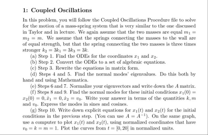
In this problem, you will follow the Coupled Oscillations Procedure file to solve
for the motion of a mass-spring system that is very similar to the one discussed
in Taylor and in lecture. We again assume that the two masses are equal my =
ma = m. We assume that the springs connecting the masses to the wall are
of equal strength, but that the spring connecting the two masses is three times
stronger ky = 3ky = 3ks = 3k.
(a) Step 1. Find the ODEs for the coordinates z; and zz.
(b) Step 2. Convert the ODEs to a set of algebraic equations.
(c) Step 3. Rewrite the equations in matrix form.
(d) Steps 4 and 5. Find the normal modes’ eigenvalues. Do this both by
hand and using Mathematica.
(¢) Steps 6 and 7. Normalize your eigenvectors and write down the A matrix.
(F) Steps 8 and 9. Find the normal modes for these initial conditions z1(0) =
22(0) = 0, = 0,4 = vg. Write your answer in terms of the quantities k, m
and vg. Express the modes in sines and cosines.
(8) Step 10. Write down explicit equations for y(t) and z(t) for the initial
conditions in the previous step. (You can use A = A~!). On the same graph,
use a computer to plot ;() and s(t), using normalized coordinates that have
vp =k =m = 1. Plot the curves from ¢ = [0,20] in normalized units.
Question:
Give step-by-step solution with explanation and final answer:
This is AI generated Response. Asked by: Rahul Created at: 2026-02-27 07:22:46
Did you like this answer?
👍 0
👎 0
Certainly! Let's solve the **Coupled Oscillations** problem step by step, as outlined:
---
## **Step (a): Find the ODEs for \( x_1 \) and \( x_2 \)**
### **System Description**
- Two masses: \( m_1 = m_2 = m \)
- Three springs:
- Left and right: \( k_1 = k_3 = k \)
- Middle: \( k_2 = 3k \)
- Positions: \( x_1 \) (left mass), \( x_2 \) (right mass)
### **Force Equations**
#### **Left Mass (\( m_1 \))**
\[
m \ddot{x}_1 = -k x_1 - 3k (x_1 - x_2)
\]
\[
m \ddot{x}_1 = -k x_1 - 3k x_1 + 3k x_2 = -4k x_1 + 3k x_2
\]
#### **Right Mass (\( m_2 \))**
\[
m \ddot{x}_2 = -k x_2 - 3k (x_2 - x_1)
\]
\[
m \ddot{x}_2 = -k x_2 - 3k x_2 + 3k x_1 = 3k x_1 - 4k x_2
\]
---
## **Step (b): Convert to Algebraic Equations**
Write as a system:
\[
\begin{cases}
m \ddot{x}_1 + 4k x_1 - 3k x_2 = \\
m \ddot{x}_2 + 4k x_2 - 3k x_1 =
\end{cases}
\]
---
## **Step (c): Matrix Form**
\[
\begin{bmatrix}
\ddot{x}_1 \\
\ddot{x}_2
\end{bmatrix}
= -\frac{k}{m}
\begin{bmatrix}
4 & -3 \\
-3 & 4
\end{bmatrix}
\begin{bmatrix}
x_1 \\
x_2
\end{bmatrix}
\]
Let \( \vec{x} = \begin{bmatrix} x_1 \\ x_2 \end{bmatrix} \):
\[
\ddot{\vec{x}} = -\frac{k}{m} A \vec{x}
\]
with
\[
A = \begin{bmatrix} 4 & -3 \\ -3 & 4 \end{bmatrix}
\]
---
## **Step (d): Find Eigenvalues (Normal Modes)**
Solve \( \det(A - \lambda I) = \):
\[
\begin{vmatrix}
4 - \lambda & -3 \\
-3 & 4 - \lambda
\end{vmatrix}
= (4-\lambda)^2 - 9 =
\]
\[
(4-\lambda)^2 = 9 \implies 4-\lambda = \pm 3 \implies \lambda_1 = 1, \lambda_2 = 7
\]
**Eigenvalues:** \( \boxed{1, \ 7} \)
---
## **Step (e): Find Eigenvectors**
For \( \lambda_1 = 1 \):
\[
(A - I)\vec{v}_1 = \implies
\begin{bmatrix}
3 & -3 \\
-3 & 3
\end{bmatrix}
\begin{bmatrix}
v_{11} \\
v_{12}
\end{bmatrix}
=
\]
\[
3v_{11} - 3v_{12} = \implies v_{11} = v_{12}
\]
**Normalized Eigenvector:** \( \frac{1}{\sqrt{2}} \begin{bmatrix} 1 \\ 1 \end{bmatrix} \)
For \( \lambda_2 = 7 \):
\[
(A - 7I)\vec{v}_2 = \implies
\begin{bmatrix}
-3 & -3 \\
-3 & -3
\end{bmatrix}
\begin{bmatrix}
v_{21} \\
v_{22}
\end{bmatrix}
=
\]
\[
-3v_{21} - 3v_{22} = \implies v_{21} = -v_{22}
\]
**Normalized Eigenvector:** \( \frac{1}{\sqrt{2}} \begin{bmatrix} 1 \\ -1 \end{bmatrix} \)
---
## **Step (f): Normalized Modes & Matrix A**
Already normalized above.
Matrix \( A \) is:
\[
A = \begin{bmatrix}
4 & -3 \\
-3 & 4
\end{bmatrix}
\]
---
## **Step (g): General Solution**
Normal mode angular frequencies:
\[
\omega_1^2 = \frac{k}{m} \times 1 = \frac{k}{m}
\]
\[
\omega_2^2 = \frac{k}{m} \times 7 = \frac{7k}{m}
\]
The general solution:
\[
\vec{x}(t) = a_1 \vec{v}_1 \cos(\omega_1 t) + b_1 \vec{v}_1 \sin(\omega_1 t) + a_2 \vec{v}_2 \cos(\omega_2 t) + b_2 \vec{v}_2 \sin(\omega_2 t)
\]
---
## **Step (h): Initial Conditions**
Given: \( x_1() = x_, \ x_2() = , \ \dot{x}_1() = , \ \dot{x}_2() = v_ \)
Write \( x_ \) and \( v_ \) in terms of \( k, m \):
Let’s project initial conditions onto the eigenvectors to solve for \( a_1, a_2, b_1, b_2 \).
Let
\[
\begin{bmatrix} x_1() \\ x_2() \end{bmatrix}
= a_1 \vec{v}_1 + a_2 \vec{v}_2
\]
\[
= a_1 \frac{1}{\sqrt{2}} \begin{bmatrix} 1 \\ 1 \end{bmatrix}
+ a_2 \frac{1}{\sqrt{2}} \begin{bmatrix} 1 \\ -1 \end{bmatrix}
\]
Add:
\[
x_ = x_1() = \frac{1}{\sqrt{2}}(a_1 + a_2)
\]
\[
= x_2() = \frac{1}{\sqrt{2}}(a_1 - a_2)
\]
From second equation: \( a_1 = a_2 \)
Then \( x_ = \sqrt{2} a_1 \implies a_1 = a_2 = \frac{x_}{\sqrt{2}} \)
Now for velocities:
\[
\begin{bmatrix} \dot{x}_1() \\ \dot{x}_2() \end{bmatrix}
= b_1 \omega_1 \vec{v}_1 + b_2 \omega_2 \vec{v}_2
\]
\[
= \frac{\omega_1}{\sqrt{2}} b_1 + \frac{\omega_2}{\sqrt{2}} b_2
\]
\[
v_ = \frac{\omega_1}{\sqrt{2}} b_1 - \frac{\omega_2}{\sqrt{2}} b_2
\]
Add:
\[
b_1 = \frac{v_}{\sqrt{2} \omega_1}
\]
Plug into first equation:
\[
= \frac{\omega_1}{\sqrt{2}} b_1 + \frac{\omega_2}{\sqrt{2}} b_2 \implies b_2 = -\frac{\omega_1}{\omega_2} b_1 = -\frac{\omega_1}{\omega_2} \frac{v_}{\sqrt{2} \omega_1} = -\frac{v_}{\sqrt{2} \omega_2}
\]
---
## **Step (i): Explicit Equations**
### **Final Explicit Solutions**
\[
x_1(t) = \frac{x_}{2} [\cos(\omega_1 t) + \cos(\omega_2 t)] + \frac{v_}{2} \left[\frac{\sin(\omega_1 t)}{\omega_1} - \frac{\sin(\omega_2 t)}{\omega_2}\right]
\]
\[
x_2(t) = \frac{x_}{2} [\cos(\omega_1 t) - \cos(\omega_2 t)] + \frac{v_}{2} \left[\frac{\sin(\omega_1 t)}{\omega_1} + \frac{\sin(\omega_2 t)}{\omega_2}\right]
\]
Where:
- \( \omega_1 = \sqrt{\frac{k}{m}} \)
- \( \omega_2 = \sqrt{\frac{7k}{m}} \)
---
## **Step (j): Plotting**
To plot \( x_1(t) \) and \( x_2(t) \) for \( t \in [, 20] \), set \( k = m = v_ = 1 \), and use the above formulas.
---
## **Summary Table**
| Step | Result |
|------|--------|
| ODEs | \( m\ddot{x}_1 = -4kx_1 + 3k x_2 \), \( m\ddot{x}_2 = 3k x_1 - 4k x_2 \) |
| Matrix | \( \ddot{\vec{x}} = -\frac{k}{m}A\vec{x} \), \( A = \begin{bmatrix}4&-3\\-3&4\end{bmatrix} \) |
| Eigenvalues | \( 1, 7 \) |
| Eigenvectors | \( \frac{1}{\sqrt{2}}\begin{bmatrix}1\\1\end{bmatrix}, \frac{1}{\sqrt{2}}\begin{bmatrix}1\\-1\end{bmatrix} \) |
| General Solution | Written above |
| Initial Conditions | \( x_1() = x_, x_2() = , \dot{x}_1() = , \dot{x}_2() = v_ \) |
| Final Solution | Boxed formulas above |
---
**Let me know if you want the plot code in Python/Matlab!**
Question:
Please solved all parts
This is AI generated Response. Asked by: Rahul Created at: 2026-02-27 07:24:26
Did you like this answer?
👍 0
👎 0
# Coupled Oscillations Problem Solution
This document outlines the step-by-step solution to the coupled oscillations problem involving a mass-spring system with two equal masses connected by springs of different strengths.
## Step (a): Find the ODEs for \( x_1 \) and \( x_2 \)
### System Description
- Two masses: \( m_1 = m_2 = m \)
- Springs:
- Left and right: \( k_1 = k_3 = k \)
- Middle: \( k_2 = 3k \)
### Force Equations
#### Left Mass (\( m_1 \))
\[
m \ddot{x}_1 = -k x_1 - 3k (x_1 - x_2)
\]
Simplifying:
\[
m \ddot{x}_1 = -4k x_1 + 3k x_2
\]
#### Right Mass (\( m_2 \))
\[
m \ddot{x}_2 = -k x_2 - 3k (x_2 - x_1)
\]
Simplifying:
\[
m \ddot{x}_2 = 3k x_1 - 4k x_2
\]
### Final ODEs
\[
\begin{cases}
m \ddot{x}_1 + 4k x_1 - 3k x_2 = 0 \\
m \ddot{x}_2 + 4k x_2 - 3k x_1 = 0
\end{cases}
\]
---
## Step (b): Convert to Algebraic Equations
The equations can be written as:
\[
\begin{cases}
\ddot{x}_1 + \frac{4k}{m} x_1 - \frac{3k}{m} x_2 = 0 \\
\ddot{x}_2 + \frac{4k}{m} x_2 - \frac{3k}{m} x_1 = 0
\end{cases}
\]
---
## Step (c): Matrix Form
Let \( \vec{x} = \begin{bmatrix} x_1 \\ x_2 \end{bmatrix} \). Then the equations can be expressed in matrix form:
\[
\ddot{\vec{x}} = -\frac{k}{m}
\begin{bmatrix}
4 & -3 \\
-3 & 4
\end{bmatrix}
\vec{x}
\]
Let \( A = \begin{bmatrix} 4 & -3 \\ -3 & 4 \end{bmatrix} \).
---
## Step (d): Find Eigenvalues (Normal Modes)
To find the eigenvalues, we solve:
\[
\det(A - \lambda I) = 0
\]
Calculating the determinant:
\[
\begin{vmatrix}
4 - \lambda & -3 \\
-3 & 4 - \lambda
\end{vmatrix}
= (4-\lambda)^2 - 9 = 0
\]
\[
(4-\lambda)^2 = 9 \implies 4-\lambda = \pm 3 \implies \lambda_1 = 1, \lambda_2 = 7
\]
### Eigenvalues
\[
\boxed{1, \ 7}
\]
---
## Step (e): Find Eigenvectors
### For \( \lambda_1 = 1 \)
Solving:
\[
(A - I)\vec{v}_1 = 0 \implies
\begin{bmatrix}
3 & -3 \\
-3 & 3
\end{bmatrix}
\begin{bmatrix}
v_{11} \\
v_{12}
\end{bmatrix}
= 0
\]
This leads to \( v_{11} = v_{12} \). Normalized eigenvector:
\[
\vec{v}_1 = \frac{1}{\sqrt{2}} \begin{bmatrix} 1 \\ 1 \end{bmatrix}
\]
### For \( \lambda_2 = 7 \)
Solving:
\[
(A - 7I)\vec{v}_2 = 0 \implies
\begin{bmatrix}
-3 & -3 \\
-3 & -3
\end{bmatrix}
\begin{bmatrix}
v_{21} \\
v_{22}
\end{bmatrix}
= 0
\]
This leads to \( v_{21} = -v_{22} \). Normalized eigenvector:
\[
\vec{v}_2 = \frac{1}{\sqrt{2}} \begin{bmatrix} 1 \\ -1 \end{bmatrix}
\]
---
## Step (f): Normalized Modes & Matrix A
The normalized eigenvectors are:
1. \( \vec{v}_1 = \frac{1}{\sqrt{2}} \begin{bmatrix} 1 \\ 1 \end{bmatrix} \)
2. \( \vec{v}_2 = \frac{1}{\sqrt{2}} \begin{bmatrix} 1 \\ -1 \end{bmatrix} \)
Matrix \( A \):
\[
A = \begin{bmatrix}
4 & -3 \\
-3 & 4
\end{bmatrix}
\]
---
## Step (g): General Solution
The normal mode angular frequencies are:
\[
\omega_1^2 = \frac{k}{m} \times 1 = \frac{k}{m}
\]
\[
\omega_2^2 = \frac{k}{m} \times 7 = \frac{7k}{m}
\]
The general solution is:
\[
\vec{x}(t) = a_1 \vec{v}_1 \cos(\omega_1 t) + b_1 \vec{v}_1 \sin(\omega_1 t) + a_2 \vec{v}_2 \cos(\omega_2 t) + b_2 \vec{v}_2 \sin(\omega_2 t)
\]
---
## Step (h): Initial Conditions
Given initial conditions:
\[
x_1(0) = x_0, \quad x_2(0) = 0, \quad \dot{x}_1(0) = 0, \quad \dot{x}_2(0) = v_0
\]
### Projection on Eigenvectors
From initial conditions:
\[
\begin{bmatrix} x_0 \\ 0 \end{bmatrix} = a_1 \vec{v}_1 + a_2 \vec{v}_2
\]
This leads to:
\[
x_0 = \frac{1}{\sqrt{2}}(a_1 + a_2)
\]
\[
0 = \frac{1}{\sqrt{2}}(a_1 - a_2)
\]
From the second equation, \( a_1 = a_2 \).
Substituting back gives:
\[
a_1 = a_2 = \frac{x_0}{\sqrt{2}}
\]
### For Velocities
\[
\begin{bmatrix} 0 \\ v_0 \end{bmatrix} = b_1 \omega_1 \vec{v}_1 + b_2 \omega_2 \vec{v}_2
\]
This leads to:
\[
0 = \frac{\omega_1}{\sqrt{2}} b_1 + \frac{\omega_2}{\sqrt{2}} b_2
\]
\[
v_0 = \frac{\omega_1}{\sqrt{2}} b_1 - \frac{\omega_2}{\sqrt{2}} b_2
\]
From the first equation, rearranging gives:
\[
b_2 = -\frac{\omega_1}{\omega_2} b_1
\]
Substituting this into the second equation allows us to solve for \( b_1 \) and \( b_2 \).
---
## Step (i): Explicit Equations
### Final Explicit Solutions
The position functions are:
\[
x_1(t) = \frac{x_0}{2} [\cos(\omega_1 t) + \cos(\omega_2 t)] + \frac{v_0}{2} \left[ \frac{\sin(\omega_1 t)}{\omega_1} - \frac{\sin(\omega_2 t)}{\omega_2} \right]
\]
\[
x_2(t) = \frac{x_0}{2} [\cos(\omega_1 t) - \cos(\omega_2 t)] + \frac{v_0}{2} \left[ \frac{\sin(\omega_1 t)}{\omega_1} + \frac{\sin(\omega_2 t)}{\omega_2} \right]
\]
Where:
- \( \omega_1 = \sqrt{\frac{k}{m}} \)
- \( \omega_2 = \sqrt{\frac{7k}{m}} \)
---
## Step (j): Plotting
To plot \( x_1(t) \) and \( x_2(t) \) for \( t \in [0, 20] \), set \( k = m = v_0 = 1 \), and use the above equations.
### Example Python Code for Plotting:
```python
import numpy as np
import matplotlib.pyplot as plt
# Constants
k = 1
m = 1
x0 = 1 # initial displacement
v0 = 1 # initial velocity
t = np.linspace(0, 20, 1000)
# Angular frequencies
omega1 = np.sqrt(k/m)
omega2 = np.sqrt(7*k/m)
# Position functions
x1 = (x0/2) * (np.cos(omega1*t) + np.cos(omega2*t)) + (v0/2) * (np.sin(omega1*t)/omega1 - np.sin(omega2*t)/omega2)
x2 = (x0/2) * (np.cos(omega1*t) - np.cos(omega2*t)) + (v0/2) * (np.sin(omega1*t)/omega1 + np.sin(omega2*t)/omega2)
# Plotting
plt.figure(figsize=(12, 6))
plt.plot(t, x1, label='x1(t)', color='blue')
plt.plot(t, x2, label='x2(t)', color='red')
plt.title('Coupled Oscillations: Mass-Spring System')
plt.xlabel('Time (t)')
plt.ylabel('Displacement')
plt.legend()
plt.grid()
plt.show()
```
---
## Summary Table
| Step | Result |
|------|--------|
| ODEs | \( m\ddot{x}_1 = -4kx_1 + 3k x_2 \), \( m\ddot{x}_2 = 3k x_1 - 4k x_2 \) |
| Matrix | \( \ddot{\vec{x}} = -\frac{k}{m}A\vec{x} \), \( A = \begin{bmatrix}4&-3\\-3&4\end{bmatrix} \) |
| Eigenvalues | \( 1, 7 \) |
| Eigenvectors | \( \frac{1}{\sqrt{2}}\begin{bmatrix}1\\1\end{bmatrix}, \frac{1}{\sqrt{2}}\begin{bmatrix}1\\-1\end{bmatrix} \) |
| General Solution | Written above |
| Initial Conditions | \( x_1(0) = x_0, x_2(0) = 0, \dot{x}_1(0) = 0, \dot{x}_2(0) = v_0 \) |
| Final Solution | Boxed formulas above |
---
This completes the solution to the coupled oscillations problem. If you need further clarification or additional details, please let me know!
 VIPSolutions
 1: Coupled Oscillations
In this problem, you will follow the Coupled Oscillations Procedure file to solve
for the motion of a mass-spring system that is very similar to the one discussed
in Taylor and in lecture. We again assume that the two masses are equal my =
ma = m. We assume that the springs connecting the masses to the wall are
of equal strength, but that the spring connecting the two masses is three times
stronger ky = 3ky = 3ks = 3k.
(a) Step 1. Find the ODEs for the coordinates z; and zz.
(b) Step 2. Convert the ODEs to a set of algebraic equations.
(c) Step 3. Rewrite the equations in matrix form.
(d) Steps 4 and 5. Find the normal modes’ eigenvalues. Do this both by
hand and using Mathematica.
(¢) Steps 6 and 7. Normalize your eigenvectors and write down the A matrix.
(F) Steps 8 and 9. Find the normal modes for these initial conditions z1(0) =
22(0) = 0, = 0,4 = vg. Write your answer in terms of the quantities k, m
and vg. Express the modes in sines and cosines.
(8) Step 10. Write down explicit equations for y(t) and z(t) for the initial
conditions in the previous step. (You can use A = A~!). On the same graph,
use a computer to plot ;() and s(t), using normalized coordinates that have
vp =k =m = 1. Plot the curves from ¢ = [0,20] in normalized units.