 VIPSolutions
Give step-by-step solution with explanation and final answer:Draw the ramp response of a DT1-plant (use the values of Kj, and T; according to the table below, dependent on your student ID number) in a proper graph with proper axes scaling, with 5cm = 1 sec for the time axis and 2cm = 1 for the output axis / y- axis. Clearly show in the graph, where Kj, and T; can be found. 4% digit 1 2 3 5 7 of student ww ID [x [7 [15] 2 [25] 3 [35] 4 [45] 5 [55] 5 digit 1 2 3 5 7 of student ID X TE ll dd id sec
Question:
Give step-by-step solution with explanation and final answer: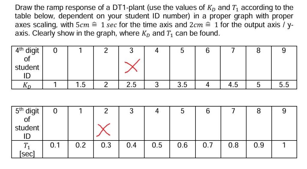 Draw the ramp response of a DT1-plant (use the values of Kj, and T; according to the
table below, dependent on your student ID number) in a proper graph with proper
axes scaling, with 5cm = 1 sec for the time axis and 2cm = 1 for the output axis / y-
axis. Clearly show in the graph, where Kj, and T; can be found.
4% digit 1 2 3 5 7
of
student ww
ID
[x [7 [15] 2 [25] 3 [35] 4 [45] 5 [55]
5 digit 1 2 3 5 7
of
student
ID X
TE ll dd id
sec
This is AI generated Response.
Asked by: Rahul
Created at: 2026-01-26 04:22:30
Asked by: Rahul
Created at: 2026-01-26 04:22:30
Final Answer:
Rendered
Raw Text
Did you like this answer?
Let's follow the instructions **step-by-step** (using the selected values from the crossed boxes in the table):
- **4th digit of student ID:** 3 → \( K_D = 2.5 \)
- **5th digit of student ID:** 2 → \( T_1 = .3 \) s
We are asked to **draw the ramp response of a DT1 system** with these values.
---
## 1. **DT1 System Transfer Function**
A DT1 system has the transfer function:
\[
G(s) = \frac{K_D}{T_1 s + 1}
\]
For a **ramp input** (\( r(t) = t \)), the Laplace transform is \( R(s) = \frac{1}{s^2} \).
The output in Laplace domain:
\[
Y(s) = G(s) \cdot R(s) = \frac{K_D}{T_1 s + 1} \cdot \frac{1}{s^2}
\]
---
## 2. **Find the Time Response**
Let's inverse Laplace:
\[
Y(s) = \frac{K_D}{T_1} \cdot \frac{1}{s^2 (s + \frac{1}{T_1})}
\]
Using partial fractions:
\[
\frac{1}{s^2 (s + a)} = \frac{A}{s} + \frac{B}{s^2} + \frac{C}{s + a}
\]
where \( a = \frac{1}{T_1} \).
Solving for \( A, B, C \):
\[
\frac{1}{s^2 (s + a)} = \frac{A}{s} + \frac{B}{s^2} + \frac{C}{s + a}
\]
\[
1 = A s (s + a) + B (s + a) + C s^2
\]
Let \( s = \): \( 1 = B \cdot a \implies B = \frac{1}{a} = T_1 \)
Let \( s = -a \): \( 1 = C a^2 \implies C = \frac{1}{a^2} = T_1^2 \)
For \( A \): Expand and collect coefficients:
\[
1 = A s (s + a) + B (s + a) + C s^2
\]
Plug in \( B = T_1, C = T_1^2 \):
\[
1 = A s (s + a) + T_1 (s + a) + T_1^2 s^2
\]
Expand:
\[
1 = A (s^2 + a s) + T_1 s + T_1 a + T_1^2 s^2
\]
\[
1 = (A + T_1^2) s^2 + (A a + T_1) s + T_1 a
\]
Match constant term: \( T_1 a = 1 \Rightarrow a = \frac{1}{T_1} \) (as before)
Match \( s \) coefficient: \( A a + T_1 = \implies A = -\frac{T_1}{a} = -T_1^2 \)
Match \( s^2 \) coefficient: \( A + T_1^2 = \implies A = -T_1^2 \) (consistent!)
So, the partial fractions:
\[
\frac{1}{s^2 (s + a)} = -T_1^2 \frac{1}{s} + T_1 \frac{1}{s^2} + T_1^2 \frac{1}{s + a}
\]
Multiply by \( \frac{K_D}{T_1} \):
\[
Y(s) = K_D \left[ -T_1 \frac{1}{s} + \frac{1}{s^2} + T_1 \frac{1}{s + a} \right]
\]
Inverse Laplace:
- \( \mathcal{L}^{-1}\left[ \frac{1}{s^2} \right] = t \)
- \( \mathcal{L}^{-1}\left[ \frac{1}{s} \right] = 1 \)
- \( \mathcal{L}^{-1}\left[ \frac{1}{s + a} \right] = e^{-a t} \)
So:
\[
y(t) = K_D \left[ -T_1 \cdot 1 + t + T_1 (1 - e^{-t/T_1}) \right]
\]
\[
y(t) = K_D \left[ t - T_1 e^{-t/T_1} \right]
\]
---
## 3. **Plug in the Values**
Given:
- \( K_D = 2.5 \)
- \( T_1 = .3 \) s
\[
y(t) = 2.5 \left[ t - .3 \cdot e^{-t/.3} \right]
\]
---
## 4. **Graphing Instructions**
- **Time axis:** \( 5\,\text{cm} \equiv 1\,\text{sec} \)
- **Output axis:** \( 2\,\text{cm} \equiv 1 \)
- **Label \( K_D \) (slope for large \( t \)) and \( T_1 \) (time constant) on the graph.**
---
## 5. **Key Points for Plot**
- At \( t = \): \( y() = 2.5[ - .3 \cdot 1] = -.75 \)
- As \( t \to \infty \): \( e^{-t/.3} \to \), \( y(t) \to 2.5 t \)
- The curve starts at \( -.75 \), then rises and approaches a straight line with slope \( 2.5 \).
---
### Example Table of Values
| \( t \) (s) | \( e^{-t/.3} \) | \( y(t) \) |
|-------------|------------------|--------------------|
| | 1 | -.75 |
| .2 | .5134 | 2.5[.2 - .3*.5134] ≈ 2.5[.2 - .154] ≈ 2.5*.046 ≈ .115 |
| .5 | .1889 | 2.5[.5 - .3*.1889] ≈ 2.5[.5 - .0567] ≈ 2.5*.443 ≈ 1.108 |
| 1. | .0357 | 2.5[1. - .3*.0357] ≈ 2.5[1. - .0107] ≈ 2.5*.989 ≈ 2.472 |
| 2. | .00127 | 2.5[2. - .3*.00127] ≈ 2.5[2. - .00038] ≈ 2.5*1.99962 ≈ 4.999 |
---
## 6. **How to Draw**
1. Draw time axis, label every 5 cm as 1 sec.
2. Draw output axis, label every 2 cm as 1.
3. Plot the starting point at \((, -.75)\).
4. Plot points for \( t = .2, .5, 1., 2. \) as above.
5. Draw a tangent for large \( t \), which is a straight line with slope \( K_D = 2.5 \).
6. Mark the time constant \( T_1 = .3 \) s (the time it takes for the exponential to decay to \( 1/e \)).
---
## 7. **Final Answer (Summary and Formula)**
**Ramp response of the DT1 system:**
\[
\boxed{
y(t) = 2.5 \left[ t - .3 \, e^{-t/.3} \right]
}
\]
- Initial value: \( y() = -.75 \)
- Slope for large \( t \): \( 2.5 \)
- Time constant: \( T_1 = .3 \) s
---
### **Graph (Description)**
- The curve starts at \( y() = -.75 \), rises quickly, and for large \( t \), becomes a straight line with slope \( 2.5 \).
- Mark \( K_D = 2.5 \) as the tangent slope.
- Mark \( T_1 = .3 \) s on the time axis to show the time constant.
---
If you want a plotted graph, let me know!
📢 Instructions:
- Ask anything relatd to above question only.
- For new Question goto :