Give step-by-step solution with explanation and final answer:BENG130 Biotransport
In-class exercises — Flow fundamentals problems
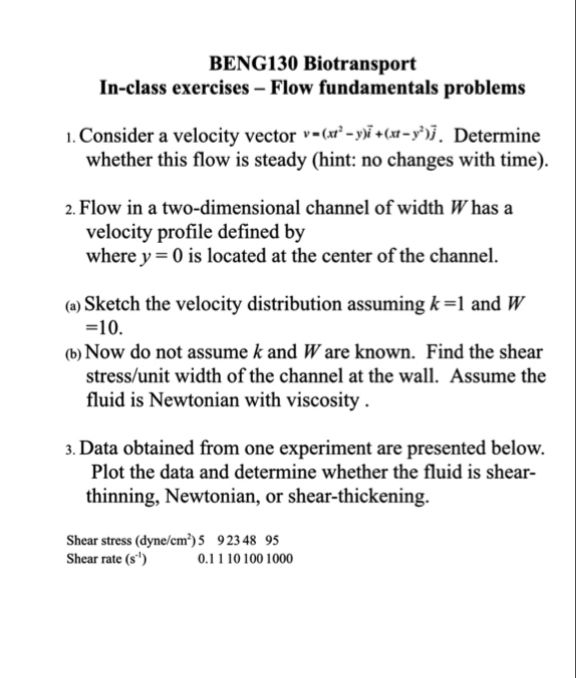
1. Consider a velocity vector v=( yi +(w-¥)j. Determine
whether this flow is steady (hint: no changes with time).
2. Flow in a two-dimensional channel of width # has a
velocity profile defined by
where y = 0 is located at the center of the channel.
(@ Sketch the velocity distribution assuming k =1 and
=10.
(Now do not assume k and are known. Find the shear
stress/unit width of the channel at the wall. Assume the
fluid is Newtonian with viscosity .
3. Data obtained from one experiment are presented below.
Plot the data and determine whether the fluid is shear-
thinning, Newtonian, or shear-thickening.
Shear stress (dyne/cm’)S 92348 95
Shear rate (s") 011101001000
Question:
Give step-by-step solution with explanation and final answer:BENG130 Biotransport
In-class exercises — Flow fundamentals problems
1. Consider a velocity vector v=( yi +(w-¥)j. Determine
whether this flow is steady (hint: no changes with time).
2. Flow in a two-dimensional channel of width # has a
velocity profile defined by
where y = 0 is located at the center of the channel.
(@ Sketch the velocity distribution assuming k =1 and
=10.
(Now do not assume k and are known. Find the shear
stress/unit width of the channel at the wall. Assume the
fluid is Newtonian with viscosity .
3. Data obtained from one experiment are presented below.
Plot the data and determine whether the fluid is shear-
thinning, Newtonian, or shear-thickening.
Shear stress (dyne/cm’)S 92348 95
Shear rate (s") 011101001000
This is AI generated Response.
Asked by: Rahul
Created at: 2026-01-24 03:11:23
Final Answer:
RenderedRaw Text
Did you like this answer?
# BENG130 Biotransport: Flow Fundamentals Problems — Step-by-Step Solutions
---
## 1. **Steadiness of the Flow**
**Given:**
\[
\vec{v} = (x^2 - y^2)\hat{i} + (x - y^2)\hat{j}
\]
**To Determine:**
Is the flow steady?
### **Solution:**
A flow is **steady** if its velocity field does **not** change with **time** (i.e., \(\partial \vec{v}/\partial t = \)).
- Here, \(\vec{v}\) depends only on \(x\) and \(y\). There is **no explicit dependence on time** (\(t\)).
- **Therefore:**
\[
\frac{\partial \vec{v}}{\partial t} =
\]
The flow is **steady**.
**Final Answer:**
\[
\boxed{\text{The flow is steady.}}
\]
---
## 2. **Velocity Profile in a Channel**
Given:
\[
v_x = k\left(1 - \left(\frac{y}{W/2}\right)^2\right)
\]
where \(y = \) at the center, and \(W\) is the channel width.
---
### (a) **Sketch the Velocity Distribution (\(k=1, W=10\))**
- \(W = 10\), so \(W/2 = 5\).
- \(v_x = 1 - \left(\frac{y}{5}\right)^2\)
- \(y\) ranges from \(-5\) to \(+5\).
**Key Points:**
- At \(y = \): \(v_x = 1\) (center, max velocity)
- At \(y = \pm 5\): \(v_x = 1 - (1)^2 = \) (walls, zero velocity)
**Sketch Description:**
- The plot is a **parabola** opening downwards, centered at \(y = \), touching the \(y\)-axis at \(y = \pm 5\).
---
### (b) **Shear Stress at the Wall (\(y = \pm W/2\)), Newtonian Fluid**
**Shear stress:**
For a Newtonian fluid,
\[
\tau = \mu \left. \frac{dv_x}{dy} \right|_{\text{wall}}
\]
**Calculate derivative:**
\[
v_x = k\left[1 - \left(\frac{y}{W/2}\right)^2\right]
\]
Let \(a = W/2\):
\[
v_x = k \left( 1 - \left(\frac{y}{a}\right)^2 \right)
\]
\[
\frac{dv_x}{dy} = k \cdot \left( -2\frac{y}{a^2} \right) = -\frac{2k}{a^2}y
\]
At \(y = a = W/2\):
\[
\left. \frac{dv_x}{dy} \right|_{y = W/2} = -\frac{2k}{a^2}a = -\frac{2k}{a}
= -\frac{2k}{W/2} = -\frac{4k}{W}
\]
**So,**
\[
\tau_{\text{wall}} = \mu \left( -\frac{4k}{W} \right)
\]
**Final Answer:**
\[
\boxed{
\tau_{\text{wall}} = -\frac{4\mu k}{W}
}
\]
(Negative sign indicates direction; magnitude is \(\frac{4\mu k}{W}\).)
---
## 3. **Experimental Data: Fluid Type Identification**
**Data Table:**
| Shear Stress (dyne/cm\(^2\)) | 5 | 9 | 23 | 48 | 95 |
|------------------------------|---|---|----|----|----|
| Shear Rate (\(s^{-1}\)) |.1| 1 | 10 |100 |100|
**To Do:**
Plot shear stress vs. shear rate and determine if the fluid is Newtonian, shear-thinning, or shear-thickening.
### **Analysis:**
- For a **Newtonian fluid**, \(\tau = \mu \dot{\gamma}\) (linear relationship).
- **Shear-thinning:** Curve flattens (concave down); slope decreases with increasing rate.
- **Shear-thickening:** Curve steepens (concave up); slope increases with increasing rate.
#### **Calculate Apparent Viscosity (\(\tau/\dot{\gamma}\)):**
| Shear Rate (\(s^{-1}\)) | .1 | 1 | 10 | 100 | 100 |
|-------------------------|-----|---|----|-----|------|
| Shear Stress (dyne/cm\(^2\)) | 5 | 9 | 23 | 48 | 95 |
| Apparent Viscosity (\(\tau/\dot{\gamma}\)) | 50 | 9 | 2.3 | .48 | .095 |
- **Viscosity decreases with increasing shear rate**.
### **Conclusion:**
- **Shear-thinning** fluid (pseudoplastic behavior).
**Final Answer:**
\[
\boxed{\text{The fluid is shear-thinning.}}
\]
---
## **Summary Table**
| Part | Final Answer |
|------|-------------|
| 1 | The flow is steady. |
| 2(a) | Parabolic velocity profile, max at center, zero at walls. |
| 2(b) | \(\tau_{\text{wall}} = -\frac{4\mu k}{W}\) |
| 3 | The fluid is shear-thinning. |
---
If you need the plot for question 3, please let me know!
VIPSolutions focuses on clear, step‑by‑step explanations so you can learn quickly. Whether you need an AI‑generated walkthrough or a short hint to get unstuck, each solution is organized for fast reading and easy review later.
Search similar questions, compare approaches, and bookmark the best answers for revision. Our goal is simple: quick, reliable study help that feels natural—not noisy.
 VIPSolutions
 BENG130 Biotransport
In-class exercises — Flow fundamentals problems
1. Consider a velocity vector v=( yi +(w-¥)j. Determine
whether this flow is steady (hint: no changes with time).
2. Flow in a two-dimensional channel of width # has a
velocity profile defined by
where y = 0 is located at the center of the channel.
(@ Sketch the velocity distribution assuming k =1 and
=10.
(Now do not assume k and are known. Find the shear
stress/unit width of the channel at the wall. Assume the
fluid is Newtonian with viscosity .
3. Data obtained from one experiment are presented below.
Plot the data and determine whether the fluid is shear-
thinning, Newtonian, or shear-thickening.
Shear stress (dyne/cm’)S 92348 95
Shear rate (s") 011101001000