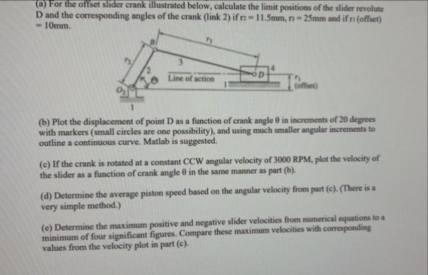
Let's break down and answer each part step by step with explanations: --- # (a) **Limit Positions of the Slider (D) and Corresponding Crank Angles** Given: - \( r_2 = 11.5\, \mathrm{mm} \) (crank, link 2) - \( r_3 = 25\, \mathrm{mm} \) (connecting rod, link 3) - \( r_1 = 10\, \mathrm{mm} \) (offset) - The slider is offset by \( r_1 \) from the origin ## **Step 1: Kinematic Loop Equation** For an offset slider-crank: - \( O_2A = r_2 \) - \( AB = r_3 \) - \( BD = x \) (slider position) - Offset = \( r_1 \) The loop closure equation (projected onto the line of action): \[ x = r_2 \cos\theta + r_3 \cos\phi \] \[ r_2 \sin\theta = r_1 + r_3 \sin\phi \] Where: - \( \theta \): Crank angle - \( \phi \): Connecting rod angle ## **Step 2: Limit Positions (Extreme Values of \( x \))** The limit positions occur when the crank and connecting rod are collinear (fully extended or fully retracted): ### **Maximum Extension:** - Crank and connecting rod aligned (to the right) - \( \theta = ^\circ \) - \( \sin\theta = , \cos\theta = 1 \) \[ r_2 \sin\theta = r_1 + r_3 \sin\phi \implies = r_1 + r_3 \sin\phi \implies \sin\phi = -\frac{r_1}{r_3} \] \[ x_{max} = r_2\cos + r_3\cos\phi_{max} \] \[ \cos\phi_{max} = \sqrt{1 - \left(-\frac{r_1}{r_3}\right)^2} \] ### **Maximum Retraction:** - Crank and connecting rod aligned (to the left) - \( \theta = 180^\circ \) - \( \sin\theta = , \cos\theta = -1 \) \[ = r_1 + r_3\sin\phi \implies \sin\phi = -\frac{r_1}{r_3} \] \[ x_{min} = -r_2 + r_3\cos\phi_{min} \] \[ \cos\phi_{min} = \sqrt{1 - \left(-\frac{r_1}{r_3}\right)^2} \] ### **Substitute Numbers:** \[ \sin\phi = -\frac{10}{25} = -.4 \] \[ \cos\phi = \sqrt{1 - .16} = \sqrt{.84} = .9165 \] **Maximum position:** \[ x_{max} = 11.5 + 25 \times .9165 = 11.5 + 22.91 = 34.41\, \text{mm} \] **Minimum position:** \[ x_{min} = -11.5 + 25 \times .9165 = -11.5 + 22.91 = 11.41\, \text{mm} \] **Corresponding angles for link 2 (crank):** - At \( x_{max} \): \( \theta = ^\circ \) - At \( x_{min} \): \( \theta = 180^\circ \) --- # (b) **Plot Displacement of Point D vs. Crank Angle \( \theta \)** ## **Step 1: General Equation** \[ r_2\sin\theta = r_1 + r_3\sin\phi \] \[ \sin\phi = \frac{r_2\sin\theta - r_1}{r_3} \] \[ \phi = \arcsin\left(\frac{r_2\sin\theta - r_1}{r_3}\right) \] \[ x = r_2\cos\theta + r_3\cos\phi \] ## **Step 2: Compute for \( \theta \) from ° to 360° in 20° increments** For each \( \theta \): 1. Calculate \( \sin\phi \) 2. Calculate \( \phi \) 3. Calculate \( x \) > **Note:** MATLAB is suggested for plotting. --- # (c) **Velocity of the Slider at 300 RPM** ## **Step 1: Angular Velocity** \[ \omega_2 = 300\,\text{RPM} \times \frac{2\pi}{60} = 314.16\, \text{rad/s} \] ## **Step 2: Instantaneous Velocity Equation** \[ \frac{dx}{dt} = -r_2 \omega_2 \sin\theta - r_3 \omega_3 \sin\phi \] But \( \omega_3 \) can be found by differentiating the loop equations. Alternatively, use: \[ \dot{x} = -r_2\omega_2\sin\theta + r_3\dot{\phi}\sin\phi \] Where \[ \dot{\phi} = \frac{r_2\omega_2\cos\theta}{r_3\cos\phi} \] So: \[ \dot{x} = -r_2\omega_2\sin\theta + r_2\omega_2\cos\theta \tan\phi \] or \[ \dot{x} = \omega_2 \left[ -r_2\sin\theta + r_2\cos\theta \tan\phi \right] \] For each \( \theta \), plug in values and plot. --- # (d) **Average Piston Speed** Average piston (slider) speed: \[ v_{avg} = \frac{2 \times (\text{Stroke}) \times (\text{RPM})}{60} \] Stroke = \( x_{max} - x_{min} = 34.41 - 11.41 = 23.00\, \text{mm} = .023\, \text{m} \) \[ v_{avg} = \frac{2 \times .023 \times 300}{60} = \frac{138}{60} = 2.3\, \text{m/s} \] --- # (e) **Maximum Positive and Negative Slider Velocities** From the velocity equation in (c), calculate the max/min values numerically (for all \( \theta \)), and compare to the analytical velocity from (c). --- ## **Final Answers (Summary):** ### (a) **Limit positions of slider D:** - \( x_{max} = \boxed{34.41\, \text{mm}} \) at \( \theta = ^\circ \) - \( x_{min} = \boxed{11.41\, \text{mm}} \) at \( \theta = 180^\circ \) ### (b) **Displacement plot:** - Use \( x(\theta) = r_2\cos\theta + r_3\cos\phi \) where \( \sin\phi = \frac{r_2\sin\theta - r_1}{r_3} \) - Plot for \( \theta \) from ° to 360° ### (c) **Slider velocity at 300 RPM:** - \( \dot{x} = \omega_2 \left[ -r_2\sin\theta + r_2\cos\theta \tan\phi \right] \), \( \omega_2 = 314.16 \) rad/s - Plot \( \dot{x} \) vs. \( \theta \) ### (d) **Average piston speed:** - \( v_{avg} = \boxed{2.3\, \text{m/s}} \) ### (e) **Maximum velocities:** - Find the max/min of \( \dot{x} \) numerically (using the formula above for all \( \theta \)), report values to 4 significant figures. --- **Let me know if you want a MATLAB script for parts (b) or (c)!**