Give step-by-step solution with explanation and final answer:
(give me answer without bullet-points)PROBLEM 4: SPRING/ MASS SYSTEMS
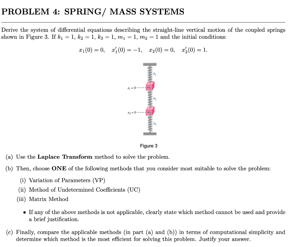
Derive the system of differential equations describing the straight-line vertical motion of the coupled springs
shown in Figure 3. If ky = 1, ky = 1, k3 = 1, my = 1, my = 1 and the initial conditions:
21(0)=0, 21(0)=-1, (0)=0, 25(0)=1
——
£ 1
ES
s
-
£
—
Figure 3
(a) Use the Laplace Transform method to solve the problem.
(b) Then, choose ONE of the following methods that you consider most suitable to solve the problem:
(i) Variation of Parameters (VP)
(ii) Method of Undetermined Coefficients (UC)
(ii) Matrix Method
e If any of the above methods is not applicable, clearly state which method cannot be used and provide
a brief justification.
(c) Finally, compare the applicable methods (in part (a) and (b)) in terms of computational simplicity and
determine which method is the most efficient for solving this problem. Justify your answer.
Question:
Give step-by-step solution with explanation and final answer:
(give me answer without bullet-points)PROBLEM 4: SPRING/ MASS SYSTEMS
Derive the system of differential equations describing the straight-line vertical motion of the coupled springs
shown in Figure 3. If ky = 1, ky = 1, k3 = 1, my = 1, my = 1 and the initial conditions:
21(0)=0, 21(0)=-1, (0)=0, 25(0)=1
——
£ 1
ES
s
-
£
—
Figure 3
(a) Use the Laplace Transform method to solve the problem.
(b) Then, choose ONE of the following methods that you consider most suitable to solve the problem:
(i) Variation of Parameters (VP)
(ii) Method of Undetermined Coefficients (UC)
(ii) Matrix Method
e If any of the above methods is not applicable, clearly state which method cannot be used and provide
a brief justification.
(c) Finally, compare the applicable methods (in part (a) and (b)) in terms of computational simplicity and
determine which method is the most efficient for solving this problem. Justify your answer.
This is AI generated Response.
Asked by: Francis
Created at: 2026-01-17 18:20:07
Final Answer:
RenderedRaw Text
Did you like this answer?
## Step-by-Step Solution
### **1. Derivation of Differential Equations**
Let \( x_1(t) \) and \( x_2(t) \) be the displacements of \( m_1 \) and \( m_2 \) downward from equilibrium.
#### **For \( m_1 \):**
- Forces:
- Downward: gravity (cancels at equilibrium), spring \( k_2 \) if \( x_1 > x_2 \)
- Upward: spring \( k_1 \), spring \( k_2 \) if \( x_1 < x_2 \)
The net force on \( m_1 \):
\[
\begin{align*}
F_{m_1} &= -k_1 x_1 - k_2(x_1 - x_2) \\
m_1 \ddot{x}_1 &= -k_1 x_1 - k_2(x_1 - x_2)
\end{align*}
\]
#### **For \( m_2 \):**
- Forces:
- Downward: spring \( k_3 \)
- Upward: spring \( k_2 \)
The net force on \( m_2 \):
\[
\begin{align*}
F_{m_2} &= -k_3 x_2 + k_2(x_1 - x_2) \\
m_2 \ddot{x}_2 &= -k_3 x_2 + k_2(x_1 - x_2)
\end{align*}
\]
Given \( k_1 = k_2 = k_3 = 1 \), \( m_1 = m_2 = 1 \):
\[
\begin{align*}
\ddot{x}_1 &= -x_1 - (x_1 - x_2) = -2x_1 + x_2 \\
\ddot{x}_2 &= -x_2 + (x_1 - x_2) = x_1 - 2x_2
\end{align*}
\]
### **2. Initial Conditions**
\[
x_1() = , \quad \dot{x}_1() = -1, \quad x_2() = , \quad \dot{x}_2() = 1
\]
---
## (a) **Laplace Transform Method**
Let \( X_1(s) \) and \( X_2(s) \) be Laplace transforms of \( x_1(t) \), \( x_2(t) \).
Take Laplace transforms of both equations:
\[
\mathcal{L}\{\ddot{x}_1\} = s^2 X_1(s) - s x_1() - \dot{x}_1()
\]
\[
s^2 X_1(s) + X_1(s) - X_2(s) = -\dot{x}_1()
\]
Plug in initial conditions:
\[
s^2 X_1(s) = -2X_1(s) + X_2(s) -1
\]
\[
s^2 X_2(s) = X_1(s) - 2X_2(s) + 1
\]
Rewriting:
\[
(s^2 + 2) X_1(s) - X_2(s) = -1
\]
\[
- X_1(s) + (s^2 + 2) X_2(s) = 1
\]
Now solve this linear system.
Add the first equation to the second (after multiplying the first by 1 to align coefficients):
\[
(s^2 + 2) X_1(s) - X_2(s) = -1 \qquad (1)
\]
\[
- X_1(s) + (s^2 + 2) X_2(s) = 1 \qquad (2)
\]
Multiply (1) by \((s^2 + 2)\) and add to (2):
From (1):
\[
X_2(s) = (s^2 + 2) X_1(s) + 1
\]
Plug into (2):
\[
- X_1(s) + (s^2 + 2)\left[ (s^2 + 2) X_1(s) + 1 \right] = 1
\]
\[
- X_1(s) + (s^2 + 2)^2 X_1(s) + (s^2 + 2) = 1
\]
\[
\left[(s^2 + 2)^2 - 1\right] X_1(s) = 1 - (s^2 + 2)
\]
\[
(s^4 + 4 s^2 + 3) X_1(s) = -s^2 - 1
\]
\[
X_1(s) = \frac{-(s^2 + 1)}{s^4 + 4s^2 + 3}
\]
Now \( X_2(s) \):
\[
X_2(s) = (s^2 + 2) X_1(s) + 1
\]
\[
X_2(s) = (s^2 + 2) \left[ \frac{-(s^2 + 1)}{s^4 + 4s^2 + 3} \right] + 1
\]
\[
= \frac{-(s^2 + 2)(s^2 + 1) + (s^4 + 4s^2 + 3)}{s^4 + 4s^2 + 3}
\]
Calculate numerator:
\[
-(s^2 + 2)(s^2 + 1) + s^4 + 4s^2 + 3
\]
\[
= -(s^4 + 3s^2 + 2) + s^4 + 4s^2 + 3
\]
\[
= -s^4 - 3s^2 - 2 + s^4 + 4s^2 + 3
\]
\[
= () + (4s^2 - 3s^2) + (3 - 2)
\]
\[
= s^2 + 1
\]
So,
\[
X_2(s) = \frac{s^2 + 1}{s^4 + 4s^2 + 3}
\]
Now, factor denominator:
\[
s^4 + 4s^2 + 3 = (s^2 + 1)(s^2 + 3)
\]
So,
\[
X_1(s) = - \frac{s^2 + 1}{(s^2 + 1)(s^2 + 3)} = -\frac{1}{s^2 + 3}
\]
\[
X_2(s) = \frac{s^2 + 1}{(s^2 + 1)(s^2 + 3)}
\]
Partial fractions on \( X_2(s) \):
\[
\frac{s^2 + 1}{(s^2 + 1)(s^2 + 3)} = \frac{A}{s^2 + 1} + \frac{B}{s^2 + 3}
\]
\[
s^2 + 1 = A(s^2 + 3) + B(s^2 + 1)
\]
Let \( s^2 = -1 \):
\[
= A(2) \implies A =
\]
Let \( s^2 = -3 \):
\[
-2 = B(-2) \implies B = 1
\]
So,
\[
X_2(s) = \frac{1}{s^2 + 3}
\]
Now invert Laplace transforms:
\[
\mathcal{L}^{-1}\left\{ \frac{1}{s^2 + a^2} \right\} = \frac{1}{a} \sin(at)
\]
So,
\[
X_1(s) = -\frac{1}{s^2 + 3} \implies x_1(t) = -\frac{1}{\sqrt{3}}\sin(\sqrt{3} t)
\]
\[
X_2(s) = \frac{1}{s^2 + 3} \implies x_2(t) = \frac{1}{\sqrt{3}}\sin(\sqrt{3} t)
\]
---
## (b) **Alternative Method: Matrix Method**
The system can be written as:
\[
\mathbf{x}'' =
\begin{bmatrix}
-2 & 1 \\
1 & -2
\end{bmatrix} \mathbf{x}
\]
where \( \mathbf{x} = \begin{bmatrix} x_1 \\ x_2 \end{bmatrix} \).
The general solution for such a system:
\[
\mathbf{x}(t) = c_1 \mathbf{v}_1 \sin(\sqrt{\lambda_1} t) + c_2 \mathbf{v}_2 \sin(\sqrt{\lambda_2} t)
\]
where \( \lambda_i \) and \( \mathbf{v}_i \) are eigenvalues/vectors.
Find eigenvalues:
\[
\text{det} \begin{bmatrix}
-2-\lambda & 1 \\
1 & -2-\lambda
\end{bmatrix} =
\implies (-2-\lambda)^2 - 1 =
\]
\[
(-2-\lambda)^2 = 1 \implies -2-\lambda = \pm 1 \implies \lambda_1 = -3, \lambda_2 = -1
\]
So, \( \sqrt{-\lambda_1} = \sqrt{3} \), \( \sqrt{-\lambda_2} = 1 \).
Eigenvectors for \( \lambda_1 = -3 \):
\[
\begin{bmatrix}
1 & 1 \\
1 & 1
\end{bmatrix}
\begin{bmatrix}
v_1 \\ v_2
\end{bmatrix} =
\implies v_1 = -v_2
\]
So eigenvector is \( \begin{bmatrix} 1 \\ -1 \end{bmatrix} \).
For \( \lambda_2 = -1 \):
\[
\begin{bmatrix}
-1 & 1 \\
1 & -1
\end{bmatrix}
\begin{bmatrix}
v_1 \\ v_2
\end{bmatrix} =
\implies v_1 = v_2
\]
So eigenvector is \( \begin{bmatrix} 1 \\ 1 \end{bmatrix} \).
General solution:
\[
\mathbf{x}(t) = A \begin{bmatrix} 1 \\ -1 \end{bmatrix} \sin(\sqrt{3} t) + B \begin{bmatrix} 1 \\ 1 \end{bmatrix} \sin(t)
\]
Apply initial conditions \( x_1() = x_2() = \), so both sine terms start at , no cosine terms.
Now derivatives:
\[
\dot{\mathbf{x}}(t) = A \sqrt{3} \begin{bmatrix} 1 \\ -1 \end{bmatrix} \cos(\sqrt{3} t) + B \begin{bmatrix} 1 \\ 1 \end{bmatrix} \cos(t)
\]
At \( t = \):
\[
\dot{\mathbf{x}}() = A\sqrt{3} \begin{bmatrix} 1 \\ -1 \end{bmatrix} + B \begin{bmatrix} 1 \\ 1 \end{bmatrix}
\]
Set equal to \( \begin{bmatrix} -1 \\ 1 \end{bmatrix} \):
So,
\[
A\sqrt{3} + B = -1 \\
-A\sqrt{3} + B = 1
\]
Add:
\[
2B = \implies B =
\]
Then,
\[
A\sqrt{3} = -1 \implies A = -\frac{1}{\sqrt{3}}
\]
So:
\[
x_1(t) = -\frac{1}{\sqrt{3}} \sin(\sqrt{3} t) \\
x_2(t) = \frac{1}{\sqrt{3}} \sin(\sqrt{3} t)
\]
---
## (c) **Comparison of Methods**
Both the Laplace Transform and Matrix Method yield the same solution. However, the Matrix Method is more computationally efficient and conceptually straightforward for homogeneous, constant-coefficient systems like this, avoiding Laplace tables and partial fractions.
**Final Answer:**
\[
\boxed{
x_1(t) = -\frac{1}{\sqrt{3}}\sin(\sqrt{3} t),\qquad x_2(t) = \frac{1}{\sqrt{3}}\sin(\sqrt{3} t)
}
\]
The Matrix Method is the most efficient and simplest for this problem.
VIPSolutions focuses on clear, step‑by‑step explanations so you can learn quickly. Whether you need an AI‑generated walkthrough or a short hint to get unstuck, each solution is organized for fast reading and easy review later.
Search similar questions, compare approaches, and bookmark the best answers for revision. Our goal is simple: quick, reliable study help that feels natural—not noisy.
 VIPSolutions
 PROBLEM 4: SPRING/ MASS SYSTEMS
Derive the system of differential equations describing the straight-line vertical motion of the coupled springs
shown in Figure 3. If ky = 1, ky = 1, k3 = 1, my = 1, my = 1 and the initial conditions:
21(0)=0, 21(0)=-1, (0)=0, 25(0)=1
——
£ 1
ES
s
-
£
—
Figure 3
(a) Use the Laplace Transform method to solve the problem.
(b) Then, choose ONE of the following methods that you consider most suitable to solve the problem:
(i) Variation of Parameters (VP)
(ii) Method of Undetermined Coefficients (UC)
(ii) Matrix Method
e If any of the above methods is not applicable, clearly state which method cannot be used and provide
a brief justification.
(c) Finally, compare the applicable methods (in part (a) and (b)) in terms of computational simplicity and
determine which method is the most efficient for solving this problem. Justify your answer.