 VIPSolutions
Give step-by-step solution with explanation and final answer: (give me answer without using bullet-points)(1) Sketch the asymptotic Bode plots of the following transfer functions by hand. (0.5 points each) a 20 (s+05)(s +5) s+5 “5+50 bE +100 s(s +20) 15(s + 50) d—— s+5
Question:
Give step-by-step solution with explanation and final answer:
(give me answer without using bullet-points)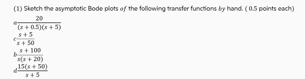 (1) Sketch the asymptotic Bode plots of the following transfer functions by hand. (0.5 points each)
a 20
(s+05)(s +5)
s+5
“5+50
bE +100
s(s +20)
15(s + 50)
d——
s+5
This is AI generated Response.
Asked by: Francis
Created at: 2026-01-17 15:52:18
Asked by: Francis
Created at: 2026-01-17 15:52:18
Final Answer:
Rendered
Raw Text
Did you like this answer?
Let's solve each transfer function step by step, explaining the procedure for drawing their **asymptotic Bode plots**. The Bode plot consists of a magnitude plot (in dB) and a phase plot (in degrees---
### (a) \(\frac{20}{(s+.5)(s+5)}\)
First, express in standard form for Bode plots:
\[
G(s) = \frac{20}{(s+.5)(s+5)}
\]
Substitute \(s = j\omega\):
\[
G(j\omega) = \frac{20}{(j\omega + .5)(j\omega + 5)}
\]
**Breakpoints (corner frequencies):**
\(\omega_1 = .5\), \(\omega_2 = 5\)
**DC gain (low-frequency gain):**
At \(\omega \ll .5\),
\[
|G(j\omega)| \approx \frac{20}{.5 \times 5} = 8
\]
Magnitude in dB: \(20 \log_{10}(8) \approx 18\) dB
**Slopes:**
- Below \(\omega_1 = .5\): slope = dB/decade.
- Between \(\omega_1\) and \(\omega_2\): slope = -20 dB/decade.
- Above \(\omega_2\): slope = -40 dB/decade.
**Phase:**
Each pole introduces -45° at its corner frequency, approaching -90° per pole at high frequency.
Total phase shift at high frequency: -180°.
---
### (b) \(\frac{s+100}{s(s+20)}\)
Rewrite:
\[
G(s) = \frac{s+100}{s(s+20)}
\]
\[
G(j\omega) = \frac{j\omega+100}{j\omega(j\omega+20)}
\]
**Zero at:** \(\omega_z = 100\)
**Poles at:** \(\omega = \) (integrator), \(\omega_p = 20\)
**DC gain:**
At \(\omega \ll 20\): numerator ≈ 100, denominator ≈ \(j\omega \cdot 20\).
**Slopes:**
- Below \(\omega_p = 20\): start with slope = -20 dB/decade (due to integrator).
- At \(\omega = 20\): another pole, add -20 dB/decade (total = -40 dB/decade).
- At \(\omega = 100\): zero, add +20 dB/decade (total = -20 dB/decade above 100).
---
### (c) \(\frac{s+5}{s+50}\)
Rewrite:
\[
G(s) = \frac{s+5}{s+50}
\]
\[
G(j\omega) = \frac{j\omega+5}{j\omega+50}
\]
**Zero at:** \(\omega_z = 5\)
**Pole at:** \(\omega_p = 50\)
**DC gain:**
At \(\omega \ll 5\), numerator ≈ 5, denominator ≈ 50, so gain = .1
Magnitude in dB: \(20\log_{10}(.1) = -20\) dB
**Slopes:**
- Below \(\omega_z = 5\): slope = dB/dec.
- From \(\omega_z = 5\): +20 dB/dec.
- From \(\omega_p = 50\): -20 dB/dec (net slope back to dB/dec above 50).
---
### (d) \(\frac{15(s+50)}{s+5}\)
Rewrite:
\[
G(s) = \frac{15(s+50)}{s+5}
\]
\[
G(j\omega) = \frac{15(j\omega+50)}{j\omega+5}
\]
**Zero at:** \(\omega_z = 50\)
**Pole at:** \(\omega_p = 5\)
**DC gain:**
At \(\omega \ll 5\), numerator ≈ 15 × 50 = 750, denominator ≈ 5, so gain = 150
Magnitude in dB: \(20\log_{10}(150) \approx 43.5\) dB
**Slopes:**
- Below \(\omega_p = 5\): slope = dB/dec.
- At \(\omega_p = 5\): -20 dB/dec.
- At \(\omega_z = 50\): +20 dB/dec (net slope back to dB/dec above 50).
---
## **Summary Table**
| Function | DC Gain (dB) | Break Frequencies | Slope Changes (dB/dec) |
|----------|:------------:|:----------------:|:-------------------------------|
| (a) | ~18 | .5, 5 | → -20 (@.5) → -40 (@5) |
| (b) | -- | , 20, 100 | -20 → -40 (@20) → -20 (@100) |
| (c) | -20 | 5, 50 | → +20 (@5) → (@50) |
| (d) | 43.5 | 5, 50 | → -20 (@5) → (@50) |
---
This is the step-by-step process for sketching the asymptotic Bode plots, including break frequencies, DC gain, and slope changes for each transfer function. The actual sketch would follow these rules for magnitude and phase.
📢 Instructions:
- Ask anything relatd to above question only.
- For new Question goto :