 VIPSolutions
Give step-by-step solution with explanation and final answer:The closed-loop block diagram of the system is given below. Calculate Kc and time constants for P, PI and PID controller by using Ziegler-Nichols controller settings and using Bode diagram. (Hint: Show all calculations in details but you can draw only the overall system’s AR and phase lag on the Bode diagram and you can use asymptotic consideration) Ys) + — 1
Question:
Give step-by-step solution with explanation and final answer: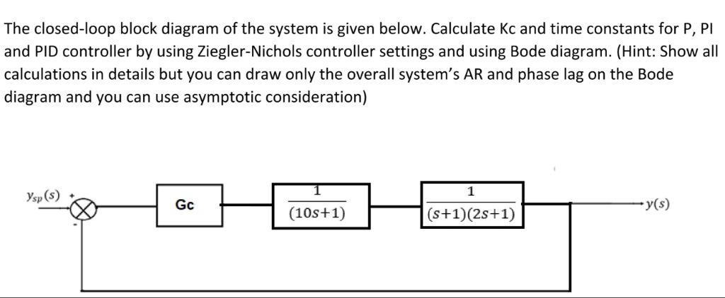 The closed-loop block diagram of the system is given below. Calculate Kc and time constants for P, PI
and PID controller by using Ziegler-Nichols controller settings and using Bode diagram. (Hint: Show all
calculations in details but you can draw only the overall system’s AR and phase lag on the Bode
diagram and you can use asymptotic consideration)
Ys) + — 1
This is AI generated Response.
Asked by: Francis
Created at: 2026-01-06 13:11:00
Asked by: Francis
Created at: 2026-01-06 13:11:00
Final Answer:
Rendered
Raw Text
Did you like this answer?
Let's break down the problem step by step, as required:
---
# 1. **Open-Loop Transfer Function**
Given system (excluding controller \( G_c \)):
\[
G(s) = \frac{1}{(10s + 1)(s + 1)(2s + 1)}
\]
If the controller gain is \( K_c \), the open-loop transfer function is:
\[
L(s) = K_c G(s) = \frac{K_c}{(10s + 1)(s + 1)(2s + 1)}
\]
---
# 2. **Bode Plot Asymptotic Analysis**
- **Poles at:** \( s = -.1, -1, -.5 \)
- **Break frequencies:** \( .1, .5, 1 \) rad/s
### **Magnitude Plot (Asymptotic)**
- Slope starts at dB/dec.
- At each pole, slope decreases by -20 dB/dec.
### **Phase Plot (Asymptotic)**
- Each pole introduces -90° phase lag, starting about a decade before the pole frequency.
---
# 3. **Ultimate Gain (\( K_u \)) and Period (\( P_u \)) via Bode Plot**
## **Step 1: Find Gain Crossover for -180° Phase**
The Ziegler-Nichols method requires:
- The gain at which the **open-loop system** has a **phase lag of -180°** and **|L(jω)| = 1 ( dB)**.
- The frequency where this happens is called the **ultimate frequency** (\( \omega_u \)), and the gain is \( K_u \).
### **Open Loop Phase Equation**
For \( G(s) \) at \( s = j\omega \):
\[
\angle G(j\omega) = -\tan^{-1}(10\omega) - \tan^{-1}(\omega) - \tan^{-1}(2\omega)
\]
Set total phase lag to -180° (or -π radians):
\[
\tan^{-1}(10\omega_u) + \tan^{-1}(\omega_u) + \tan^{-1}(2\omega_u) = 180°
\]
Or, since each arctan is positive for ω > , their sum should be 180°:
\[
\tan^{-1}(10\omega_u) + \tan^{-1}(\omega_u) + \tan^{-1}(2\omega_u) = 180°
\]
But each arctan maxes out at 90°, so let's check possible ω numerically:
#### Try ω = 1:
- \( \tan^{-1}(10) \approx 84.3° \)
- \( \tan^{-1}(1) = 45° \)
- \( \tan^{-1}(2) \approx 63.4° \)
- **Sum = 84.3 + 45 + 63.4 ≈ 192.7°** (too high)
#### Try ω = .5:
- \( \tan^{-1}(5) \approx 78.7° \)
- \( \tan^{-1}(.5) \approx 26.6° \)
- \( \tan^{-1}(1) = 45° \)
- **Sum = 78.7 + 26.6 + 45 ≈ 150.3°** (too low)
#### Try ω = .7:
- \( \tan^{-1}(7) \approx 81.9° \)
- \( \tan^{-1}(.7) \approx 34.99° \)
- \( \tan^{-1}(1.4) \approx 54.5° \)
- **Sum = 81.9 + 35 + 54.5 ≈ 171.4°**
#### Try ω = .8:
- \( \tan^{-1}(8) \approx 82.9° \)
- \( \tan^{-1}(.8) \approx 38.7° \)
- \( \tan^{-1}(1.6) \approx 58.° \)
- **Sum = 82.9 + 38.7 + 58 ≈ 179.6°**
So, **at ω ≈ .8 rad/s, phase lag is about -180°.**
---
# 4. **Find Ultimate Gain (\( K_u \))**
At \( \omega_u = .8 \):
\[
|G(j\omega_u)| = \left| \frac{1}{(j8+1)(j.8+1)(j1.6+1)} \right|
\]
Compute each term's magnitude:
- \( |j8+1| = \sqrt{8^2+1^2} = \sqrt{65} \approx 8.06 \)
- \( |j.8+1| = \sqrt{.8^2+1^2} = \sqrt{1.64} \approx 1.28 \)
- \( |j1.6+1| = \sqrt{1.6^2+1^2} = \sqrt{3.56} \approx 1.89 \)
So,
\[
|G(j.8)| = \frac{1}{8.06 \times 1.28 \times 1.89} \approx \frac{1}{19.51} \approx .0512
\]
For critical gain (|L(jω)| = 1):
\[
K_u \cdot .0512 = 1 \implies K_u = \frac{1}{.0512} \approx 19.53
\]
---
# 5. **Ultimate Period (\( P_u \))**
\[
P_u = \frac{2\pi}{\omega_u} = \frac{2\pi}{.8} \approx 7.85
\]
---
# 6. **Ziegler-Nichols Tuning Formulas**
| Controller | \( K_c \) | \( \tau_I \) (Integral Time) | \( \tau_D \) (Derivative Time) |
|------------|-------------------|------------------------------|---------------------------------|
| P | .5 \( K_u \) | — | — |
| PI | .45 \( K_u \) | \( P_u / 1.2 \) | — |
| PID | .6 \( K_u \) | \( P_u / 2 \) | \( P_u / 8 \) |
### **Substitute values:**
- \( K_u \approx 19.53 \)
- \( P_u \approx 7.85 \)
#### **P Controller:**
- \( K_c = .5 \times 19.53 = 9.77 \)
#### **PI Controller:**
- \( K_c = .45 \times 19.53 = 8.79 \)
- \( \tau_I = P_u / 1.2 = 7.85 / 1.2 = 6.54 \)
#### **PID Controller:**
- \( K_c = .6 \times 19.53 = 11.72 \)
- \( \tau_I = 7.85 / 2 = 3.93 \)
- \( \tau_D = 7.85 / 8 = .98 \)
---
# 7. **Summary Table**
| Controller | \( K_c \) | \( \tau_I \) | \( \tau_D \) |
|------------|-----------|--------------|--------------|
| P | 9.77 | — | — |
| PI | 8.79 | 6.54 | — |
| PID | 11.72 | 3.93 | .98 |
---
# 8. **Bode Plot (Asymptotic)**
- **Magnitude:** Start at dB, slope decreases by -20 dB/dec at each break frequency (.1, .5, 1 rad/s).
- **Phase:** Each pole introduces -90° lag, total -270° for high frequencies.
- **Critical frequency:** At ω ≈ .8 rad/s, phase lag ≈ -180°.
---
## **Final Answers**
**Proportional Controller:**
- \( K_c = 9.77 \)
**PI Controller:**
- \( K_c = 8.79, \quad \tau_I = 6.54 \)
**PID Controller:**
- \( K_c = 11.72, \quad \tau_I = 3.93, \quad \tau_D = .98 \)
---
### **If you need a sketch of the Bode diagram, let me know!**
📢 Instructions:
- Ask anything relatd to above question only.
- For new Question goto :