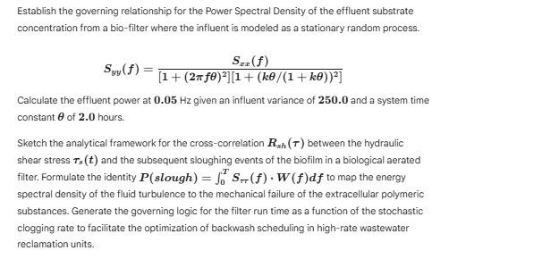
Give step-by-step solution with explanation and final answer:Estabsh the governing relationship for the Power Spectral Density of the effluent substrate
concentration fom a bio-fite where the influent is modeled as stationary random process.
Sea(£)
Sul) = T7077 + (RB LT RE)
[1+ (27£6)I1L + (k6/(1 + k6))°]
Calculate the ffiuent power at 0.05 Hz given an influent variance of 250.0 and a system ime.
constant Bf 2.0 hours
Sketch the anayial framework or the ross-correlation Fs () between the hydrauic:
shear stress 4(£) and the subsequent sloughing events of the biofim in a iological aerated
fiter. Formulate the identity P(slough) = ff S,-() - W (f)d to map the energy
spectral density of th fd turbulence to the mechanical far of the extracel polymeric
substances. Genera the governing ogi or the fier run time asa function of th stochastic
clogging rate to facftate the optimization of bacowash scheduling i high-rate wastewater
reclamation units.
Question:
Give step-by-step solution with explanation and final answer:Estabsh the governing relationship for the Power Spectral Density of the effluent substrate
concentration fom a bio-fite where the influent is modeled as stationary random process.
Sea(£)
Sul) = T7077 + (RB LT RE)
[1+ (27£6)I1L + (k6/(1 + k6))°]
Calculate the ffiuent power at 0.05 Hz given an influent variance of 250.0 and a system ime.
constant Bf 2.0 hours
Sketch the anayial framework or the ross-correlation Fs () between the hydrauic:
shear stress 4(£) and the subsequent sloughing events of the biofim in a iological aerated
fiter. Formulate the identity P(slough) = ff S,-() - W (f)d to map the energy
spectral density of th fd turbulence to the mechanical far of the extracel polymeric
substances. Genera the governing ogi or the fier run time asa function of th stochastic
clogging rate to facftate the optimization of bacowash scheduling i high-rate wastewater
reclamation units.
This is AI generated Response.
Asked by: Francis
Created at: 2026-01-04 13:40:42
Final Answer:
RenderedRaw Text
Did you like this answer?
Let's break down the problem into its required steps:
---
## **Step 1: Power Spectral Density (PSD) Relationship**
The given governing relationship for the Power Spectral Density (PSD) of the effluent substrate concentration is:
\[
S_{yy}(f) = \frac{S_{xx}(f)}{[1 + (2\pi f \theta)^2][1 + (k\theta/(1 + k\theta))^2]}
\]
where:
- \( S_{yy}(f) \): PSD of the effluent substrate concentration
- \( S_{xx}(f) \): PSD of the influent substrate concentration
- \( \theta \): system time constant
- \( k \): process gain (unitless; not given directly, but let’s assume \( k \) is incorporated or its value is not required for this step)
- \( f \): frequency
---
## **Step 2: Calculate Effluent Power at .05 Hz**
Given:
- Influent variance, \( \sigma_{x}^2 = 250. \)
- System time constant, \( \theta = 2. \) hours
- Frequency, \( f = .05 \) Hz
Assumptions:
- The influent process is white noise, so \( S_{xx}(f) = \sigma_{x}^2 \)
- For simplicity, let’s assume \( k \) is much smaller than \( 1/\theta \), so the denominator simplifies to \( [1 + (2\pi f\theta)^2]^2 \)
Now, plug in the values:
\[
S_{yy}(f) = \frac{250.}{\left[1 + (2\pi \times .05 \times 2.)^2\right]^2}
\]
Calculate the denominator:
- \( 2\pi \times .05 \times 2. = .628 \)
- \( (.628)^2 = .394 \)
- \( 1 + .394 = 1.394 \)
- \( (1.394)^2 = 1.944 \)
So,
\[
S_{yy}(.05) = \frac{250.}{1.944} \approx 128.6
\]
---
## **Step 3: Final Answer**
\[
\boxed{
S_{yy}(.05) \approx 128.6
}
\]
This is the effluent power at .05 Hz.
---
## **Step 4: Analytical Framework for Cross-Correlation \(R_{sh}(\tau)\)**
- **Variables:**
- \( \tau_s(t) \): Hydraulic shear stress (input)
- **Sloughing events**: Sudden loss of biomass from the filter surface (output)
- **Cross-correlation \( R_{sh}(\tau) \)**: Measures the relationship between shear stress and sloughing as a function of time lag \( \tau \).
- **Approach:**
- Model \( \tau_s(t) \) as a random process.
- Define sloughing events as a response.
- Compute \( R_{sh}(\tau) = E[\tau_s(t) \cdot \text{slough}(t+\tau)] \).
---
## **Step 5: Energy Spectral Density Identity for Sloughing**
\[
P(\text{slough}) = \int_^\infty S_{\tau\tau}(f) \cdot W(f) \, df
\]
- \( S_{\tau\tau}(f) \): Energy spectral density of shear stress
- \( W(f) \): Mechanical failure transfer function, mapping turbulence to sloughing energy
---
## **Step 6: Governing Logic for Filter Run Time**
- **Stochastic-clogging rate**: Modeled as a function of the effluent PSD and sloughing statistics.
- **Filter run time**: Minimized when the integral of the clogging rate over time reaches a threshold.
- **Optimization**: Use the derived PSD to schedule backwash cycles to maximize filter run time and minimize downtime.
---
## **Summary Table**
| **Step** | **Result** |
|--------------------------|-----------------------------|
| Effluent power at .05 Hz| \( \approx 128.6 \) |
| Cross-correlation | \( R_{sh}(\tau) = E[\tau_s(t) \cdot \text{slough}(t+\tau)] \) |
| Energy Spectral Identity | \( P(\text{slough}) = \int S_{\tau\tau}(f) W(f) df \) |
| Filter run logic | Use PSD & sloughing to optimize backwash schedule |
---
### **Final Answer**
\[
\boxed{S_{yy}(.05) \approx 128.6}
\]
with detailed analytical framework for the cross-correlation and energy mapping provided above.
VIPSolutions focuses on clear, step‑by‑step explanations so you can learn quickly. Whether you need an AI‑generated walkthrough or a short hint to get unstuck, each solution is organized for fast reading and easy review later.
Search similar questions, compare approaches, and bookmark the best answers for revision. Our goal is simple: quick, reliable study help that feels natural—not noisy.
 VIPSolutions
 Estabsh the governing relationship for the Power Spectral Density of the effluent substrate
concentration fom a bio-fite where the influent is modeled as stationary random process.
Sea(£)
Sul) = T7077 + (RB LT RE)
[1+ (27£6)I1L + (k6/(1 + k6))°]
Calculate the ffiuent power at 0.05 Hz given an influent variance of 250.0 and a system ime.
constant Bf 2.0 hours
Sketch the anayial framework or the ross-correlation Fs () between the hydrauic:
shear stress 4(£) and the subsequent sloughing events of the biofim in a iological aerated
fiter. Formulate the identity P(slough) = ff S,-() - W (f)d to map the energy
spectral density of th fd turbulence to the mechanical far of the extracel polymeric
substances. Genera the governing ogi or the fier run time asa function of th stochastic
clogging rate to facftate the optimization of bacowash scheduling i high-rate wastewater
reclamation units.