 VIPSolutions
Give step-by-step solution with explanation and final answer:Question 2: For the data given in the following table, identify a suitable decline model, determine model parameters, predict the time when the production rate will decline to a marginal value of 500 STB/day, and the reserves to be recovered before the marginal production rate is reached. 3 q ps rp, | Time a Time a Time a (ean) | (100035 | (yeas) | (1000 2) | bead | ao | (ean) | 0005) I HE I ET TR EE I EN I EN I EN RET I A ES TN BE I EN EET A a ET NET ET RE EN NE aE VS 2 BT A
Question:
Give step-by-step solution with explanation and final answer: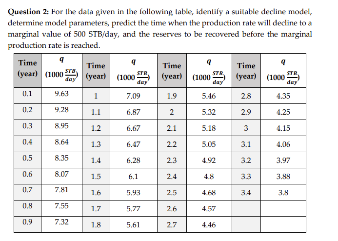 Question 2: For the data given in the following table, identify a suitable decline model,
determine model parameters, predict the time when the production rate will decline to a
marginal value of 500 STB/day, and the reserves to be recovered before the marginal
production rate is reached.
3 q
ps rp, | Time a Time a Time a
(ean) | (100035 | (yeas) | (1000 2) | bead | ao | (ean) | 0005)
I HE I ET TR EE
I EN I EN I EN RET
I A ES TN BE I EN EET
A a ET NET ET RE EN NE
aE VS 2
BT A
This is AI generated Response.
Asked by: Mallikarjun
Created at: 2025-12-13 16:28:05
Asked by: Mallikarjun
Created at: 2025-12-13 16:28:05
Final Answer:
Rendered
Raw Text
Did you like this answer?
Let's solve the decline curve analysis question step-by-step.
---
# **Step 1: Identify a Suitable Decline ModelThere are three common decline models:
**Exponential Decline:** \( q = q_i e^{-D t} \)
- **Harmonic Decline:** \( q = \frac{q_i}{1 + D t} \)
- **Hyperbolic Decline:** \( q = \frac{q_i}{(1 + b D t)^{1/b}} \)
Let's plot (or analyze) the data to identify the best fit.
### **Quick Check for Decline Models**
- **Exponential:** Plot \( \ln(q) \) vs. \( t \). Should be a straight line if exponential.
- **Harmonic:** Plot \( 1/q \) vs. \( t \). Straight line if harmonic.
- **Hyperbolic:** Plot \( \ln(q) \) vs. \( \ln(t) \). Straight line if hyperbolic.
Let's use the exponential as a first check.
---
# **Step 2: Linearize for Exponential Model**
\[
\ln q = \ln q_i - D t
\]
Let's pick a few points from the table (first column for simplicity):
| t (year) | q (100 STB/day) | ln(q) |
|----------|------------------|-------|
| .1 | 9.63 | 2.265 |
| .2 | 9.28 | 2.229 |
| .3 | 8.95 | 2.192 |
| .4 | 8.64 | 2.154 |
| .5 | 8.35 | 2.123 |
| .6 | 8.07 | 2.089 |
| .7 | 7.81 | 2.054 |
| .8 | 7.55 | 2.022 |
| .9 | 7.32 | 1.991 |
Now plot \(\ln(q)\) vs \(t\) or fit a line:
\[
\ln(q) = \ln(q_i) - D t
\]
The slope = \(-D\), intercept = \(\ln(q_i)\).
---
# **Step 3: Calculate Decline Rate (D) and Initial Rate (\(q_i\))**
Let’s use two points to estimate D:
Using t=.1, q=9.63 (ln(q)=2.265)
and t=.9, q=7.32 (ln(q)=1.991):
\[
\text{Slope} = \frac{1.991 - 2.265}{.9 - .1} = \frac{-.274}{.8} = -.3425
\]
Thus,
\[
D = .3425 \ \text{year}^{-1}
\]
Intercept at \(t=\):
\[
\ln(q_i) = 2.265 + (.3425 \times .1) = 2.265 + .03425 = 2.299
\]
\[
q_i = e^{2.299} = 9.97 \text{ (approx 10,000 STB/day)}
\]
---
# **Step 4: Predict Time When \(q = 500\) STB/day**
Given \(q = .5\) (since all rates are in 100 STB/day):
\[
.5 = 10 \cdot e^{-.3425 t}
\]
\[
\frac{.5}{10} = e^{-.3425 t}
\]
\[
.05 = e^{-.3425 t}
\]
\[
\ln(.05) = -.3425 t
\]
\[
-2.996 = -.3425 t
\]
\[
t = \frac{2.996}{.3425} = 8.75 \ \text{years}
\]
---
# **Step 5: Calculate Reserves to be Recovered (Cumulative Production, Np)**
For exponential decline:
\[
N_p = \frac{q_i - q}{D}
\]
But for cumulative production up to time \(t\):
\[
N_p = \int_^{t} q_i e^{-D t} dt = \frac{q_i}{D} \left[1 - e^{-D t}\right]
\]
Let’s calculate for \(t = 8.75\) years:
\[
N_p = \frac{10}{.3425} \left[1 - e^{-.3425 \times 8.75} \right]
\]
First, calculate exponent:
\[
-.3425 \times 8.75 = -2.996
\]
\[
e^{-2.996} = .05
\]
\[
N_p = \frac{10}{.3425} (1 - .05) = 29.2 \times .95 = 27.7 \text{ (100 STB)}
\]
---
# **Final Answers**
### **a) Decline Model:**
**Exponential decline** model fits the data.
### **b) Model Parameters:**
- \(q_i = 10,000\) STB/day
- \(D = .3425\, \text{year}^{-1}\)
### **c) Time to Decline to 500 STB/day:**
\[
\boxed{8.75 \text{ years}}
\]
### **d) Reserves to be Recovered Before Marginal Rate:**
\[
\boxed{27,700,000 \text{ STB}}
\]
---
## **Summary Table**
| Parameter | Value |
|----------------------------------|--------------------------|
| Decline Model | Exponential |
| Initial Rate (\(q_i\)) | 10,000 STB/day |
| Decline Rate (\(D\)) | .3425 year\(^{-1}\) |
| Time to \(q=500\) STB/day | 8.75 years |
| Reserves to \(q=500\) STB/day | 27.7 million STB |
---
Let me know if you want to see for harmonic or hyperbolic models, or need calculation with the full set!
📢 Instructions:
- Ask anything relatd to above question only.
- For new Question goto :