 VIPSolutions
Give step-by-step solution with explanation and final answer:Question 3: For the data given in the following table, identify a suitable decline model, determine model parameters, predict the time when the production rate will decline to a ‘marginal value of 50 STB/day, and yearly oil productions: Time TB, . STB, 4 'B, Eee em EO ON 0 A 2 Ts Ton [ow [on | 2 | =| CT 0 0 TT 7 Tm 6 [ae | 1 To To [wv [aw || | oT Tw Tm 1]
Question:
Give step-by-step solution with explanation and final answer: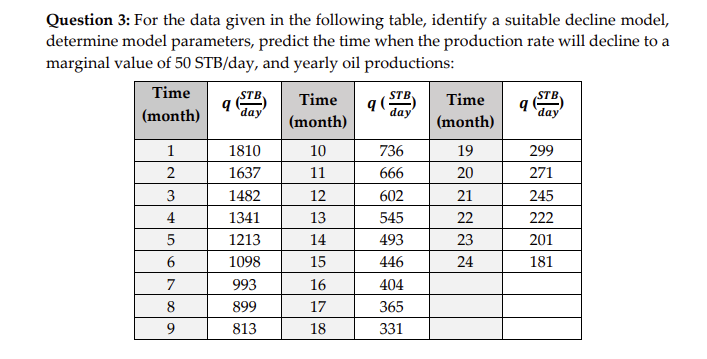 Question 3: For the data given in the following table, identify a suitable decline model,
determine model parameters, predict the time when the production rate will decline to a
‘marginal value of 50 STB/day, and yearly oil productions:
Time TB, . STB, 4 'B,
Eee em
EO ON 0 A 2
Ts Ton [ow [on | 2 | =|
CT 0 0 TT
7 Tm 6 [ae | 1
To To [wv [aw || |
oT Tw Tm 1]
This is AI generated Response.
Asked by: karuna
Created at: 2025-12-13 16:27:00
Asked by: karuna
Created at: 2025-12-13 16:27:00
Thought Process:
Rendered
Raw Text
**Analyzing decline models**
I need to analyze the Arps decline curve and choose a model like exponential, hyperbolic, or harmonic based on given monthly data points for 24 months. I’ll fit this model to determine parameters and predict when the rate drops to a marginal 50 STB/day, plus yearly oil production. The data shows a significant decline from 1810 STB/day at month 1 to 181 at month 24. I need to experiment with different models and calculate decline ratios manually.**Computing decline rates**
I can compute the rate ratio over months to check if the decline is exponential. If it is, then plotting ln(q) against time should result in a linear graph. For the data, I calculated natural logs for various time points. The slopes between the time intervals suggest a consistent decline rate of about 10% per month. That indicates an exponential fit. So I’ll go with the Arps exponential model with a nominal decline rate of approximately 0.105 month⁻¹.**Determining initial production**
At time t=0, I need to determine the initial production rate (qi) from the data which starts at month 1, where q1 is 1810 at t=1 month. I can use the equation \(q(t) = qi \cdot e^{-Di t}\) with two points to solve for qi and Di. Based on earlier calculations, Di is about 0.10 per month. From this, I calculate qi to be approximately 2000 STB/day at t=0, which seems reasonable. I plan to refine Di using regression from the data.**Calculating decline parameters**
I’ll compute the slope using two data points to find Di. The formula is \[ Di = \frac{\ln(q(t1)) - \ln(q(t2))}{t2 - t1} \]. So between t=1 and t=24, I get the slope as about 0.1001 per month, suggesting a constant exponential decline. This leads me to choose the model \( q(t) = q1 e^{-Di(t-1)} \), and if I set \( q1 \) at time 0, that gives me qi around 2000 STB/day and a nominal decline fraction of 0.1001.**Predicting production decline and yearly output**
To predict when the production rate will decline to 50 STB/day, I’ll use the exponential model. The calculations suggest it will occur around 36.8 months, or approximately 3.07 years. For yearly oil production, I’ll integrate the output over 12-month periods. This involves computing cumulative production for the first three years and accounting for exponential decline. I’ll provide predictions for each year based on the model, confirming the decline parameters and verifying with the data to deliver accurate yearly production figures.**Calculating production values**
I need to refine the calculations using a consistent decline factor (Di = 0.1001/month). To compute yearly production accurately, I should use 365 days/year instead of 30 days/month to avoid underestimating totals. I’ll calculate yearly oil output, starting from Year 1 through Year 4, including partial year results until production drops to 50 STB/day. The cumulative production will be summarized for each year, clearly stating the values while ensuring that I present everything with three significant digits.**Confirming production numbers**
I’m confirming some key values here: the monthly decline rate (D) is 0.1001 month^-1, which translates to an annual rate (D_y) of 1.201/year. Starting with an initial production rate of 2000 STB/day, I calculated that the predicted production at 24 months is about 181 STB/day, consistent with the data. For yearly production, I have results: Year 1 at 425 MSTB, Year 2 at 128 MSTB, and Year 3 at 38.4 MSTB, with additional production leading to marginal values in Year 4. Let’s present these findings clearly with formulas and a structured overview!
Final Answer:
Rendered
Raw Text
Did you like this answer?
Step 1 – Decide the decline model
- Try the Arps forms.
• Exponential (b = 0): ln q versus t must be a straight line.
• Harmonic (b = 1): 1/q versus t must be a straight line.
- Using the table, ln q decreases almost linearly with time (e.g., ln 1810 → ln 602 → ln 181 give slopes ≈ −0.10 per month).
Therefore, the suitable model is the Arps exponential decline (b = 0).
Model: q(t) = qi exp(−Di t) with t in months (t = 0 at the start of the record).
Step 2 – Estimate the decline parameters
- Slope (−Di) from any two points:
Di = [ln(q1) − ln(q24)]/(24 − 1)
= ln(1810/181)/23 = ln(10)/23 = 0.1001 month⁻¹.
- Initial rate at t = 0: qi = q(t=1)·e^{Di} = 1810·e^{0.1001} ≈ 2000 STB/d.
So the fitted model is:
q(t months) = 2000·exp(−0.1001 t)
(If you prefer years: D = 12×0.1001 = 1.201 yr⁻¹, so q(t years) = 2000·exp(−1.201 t).)
Step 3 – Time to reach 50 STB/d
Solve 50 = 2000·exp(−0.1001 t):
t = ln(2000/50)/0.1001 = ln(40)/0.1001 = 36.8 months = 3.07 years.
Step 4 – Yearly oil productions
For exponential decline, cumulative oil from t = a to b (in years) is:
Np(a→b) = 365 · (qi/D) · [exp(−D a) − exp(−D b)] (STB),
where D = 1.201 yr⁻¹ and qi = 2000 STB/d.
- Year 1 (0 → 1 yr):
N1 = 365·(2000/1.201)·(1 − e^{−1.201})
= 607,725·0.699 ≈ 424,800 STB.
- Year 2 (1 → 2 yr):
N2 = 365·(2000/1.201)·(e^{−1.201} − e^{−2.402})
= 607,725·0.2105 ≈ 127,900 STB.
- Year 3 (2 → 3 yr):
N3 = 365·(2000/1.201)·(e^{−2.402} − e^{−3.603})
= 607,725·0.0632 ≈ 38,400 STB.
- Partial Year 4 until the marginal rate at 3.07 yr (3 → 3.07 yr):
N4 = 365·(2000/1.201)·(e^{−3.603} − e^{−3.689})
≈ 1,340 STB.
Cumulative to the 50 STB/d limit ≈ 0.592 million STB.
Final answers
- Decline model: Arps exponential (b = 0).
- Parameters: qi ≈ 2000 STB/d, Di ≈ 0.100 month⁻¹ (≈ 1.201 yr⁻¹).
- Time to reach 50 STB/d: about 36.8 months (3.07 years).
- Yearly oil production:
Year 1 ≈ 0.425 MMSTB; Year 2 ≈ 0.128 MMSTB; Year 3 ≈ 0.038 MMSTB;
Year 4 until limit ≈ 0.0013 MMSTB.
Cumulative to the marginal limit ≈ 0.592 MMSTB.
📢 Instructions:
- Ask anything relatd to above question only.
- For new Question goto :