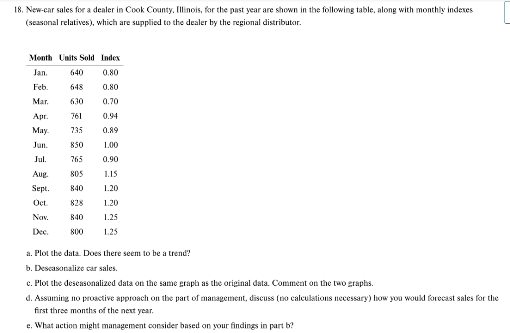
give step by step answer and give final summary18. New-car sales for a dealer in Cook County, Illinois, for the past year are shown in the following table, along with monthly indexes |
(seasonal relatives), which are supplied to the dealer by the regional distributor.
Month Units Sold Index
Jan. 640 0.80
Feb. 648 0.80
Mar. 630 0.70
Apr. 761 0.94
May. 735 0.89
Jun. 850 1.00
Jul. 765 0.90
Aug 805 115
Sept. 840 1.20
Oct. 828 120
Nov. 840 125
Dec. 800 125
a. Plot the data. Does there seem to be a trend?
b. Deseasonalize car sales.
c. Plot the deseasonalized data on the same graph as the original data. Comment on the two graphs.
d. Assuming no proactive approach on the part of management, discuss (no calculations necessary) how you would forecast sales for the
first three months of the next year.
e. What action might management consider based on your findings in part b?
Question:
give step by step answer and give final summary18. New-car sales for a dealer in Cook County, Illinois, for the past year are shown in the following table, along with monthly indexes |
(seasonal relatives), which are supplied to the dealer by the regional distributor.
Month Units Sold Index
Jan. 640 0.80
Feb. 648 0.80
Mar. 630 0.70
Apr. 761 0.94
May. 735 0.89
Jun. 850 1.00
Jul. 765 0.90
Aug 805 115
Sept. 840 1.20
Oct. 828 120
Nov. 840 125
Dec. 800 125
a. Plot the data. Does there seem to be a trend?
b. Deseasonalize car sales.
c. Plot the deseasonalized data on the same graph as the original data. Comment on the two graphs.
d. Assuming no proactive approach on the part of management, discuss (no calculations necessary) how you would forecast sales for the
first three months of the next year.
e. What action might management consider based on your findings in part b?
This is AI generated Response.
Asked by: sreegeeth
Created at: 2025-09-18 16:12:40
Final Answer:
RenderedRaw Text
Did you like this answer?
# Step-by-Step Solution
Let's address each part one by one, with clear steps and a summary at the end.
---
## a. Plot the data. Does there seem to be a trend?
**Units Sold by Month:**
| Month | Units Sold |
|-------|------------|
| Jan | 640 |
| Feb | 648 |
| Mar | 630 |
| Apr | 761 |
| May | 735 |
| Jun | 850 |
| Jul | 765 |
| Aug | 805 |
| Sept | 840 |
| Oct | 828 |
| Nov | 840 |
| Dec | 800 |
**Visual Trend Analysis:**
- Early months (Jan-Mar): Lower sales (~630-648).
- Middle months (Apr-Jul): Increasing sales, peaking in June (850), then slight drop.
- Late months (Aug-Dec): Higher sales (mostly above 800).
- **Trend:** There appears to be an upward trend from Jan to June, slight dip in July, then generally higher sales from August onward.
---
## b. Deseasonalize car sales
**Deseasonalized Sales = Units Sold / Index**
| Month | Units Sold | Index | Deseasonalized Sales |
|-------|------------|-------|----------------------|
| Jan | 640 | 0.80 | 800 |
| Feb | 648 | 0.80 | 810 |
| Mar | 630 | 0.70 | 900 |
| Apr | 761 | 0.94 | 810 |
| May | 735 | 0.89 | 825 |
| Jun | 850 | 1.00 | 850 |
| Jul | 765 | 0.90 | 850 |
| Aug | 805 | 1.15 | 700 |
| Sept | 840 | 1.20 | 700 |
| Oct | 828 | 1.20 | 690 |
| Nov | 840 | 1.25 | 672 |
| Dec | 800 | 1.25 | 640 |
---
## c. Plot the deseasonalized data on the same graph as the original data. Comment.
**Graph Comment:**
- The **original data** shows a clear seasonal pattern: low in winter, high in late summer/fall.
- The **deseasonalized data** is much flatter, showing a slight decline from Mar-Jun peak (900-850) toward year-end (640).
- **Comment:** Deseasonalizing removes the regular seasonal "ups and downs", clarifying any underlying trend (here, a slight downward trend after mid-year).
---
## d. Forecasting sales for the first three months of next year
**Method:**
- Use the average of the last few deseasonalized values (or the entire year's average) as the forecast for the base level.
- Multiply by the seasonal index for Jan, Feb, Mar.
**Example Approach:**
- Find average deseasonalized sales:
\[
\text{Average} = \frac{800 + 810 + 900 + 810 + 825 + 850 + 850 + 700 + 700 + 690 + 672 + 640}{12} \approx 771.6
\]
- Forecast for:
- **Jan:** \( 771.6 \times 0.80 \approx 617 \)
- **Feb:** \( 771.6 \times 0.80 \approx 617 \)
- **Mar:** \( 771.6 \times 0.70 \approx 540 \)
---
## e. What action might management consider based on your findings in part b?
**Findings from part b:**
- Deseasonalized data suggests a possible slight downward trend after the middle of the year.
**Management Actions:**
- Investigate reasons for the mid-to-late-year decline.
- Plan marketing or promotional efforts to boost sales in late months.
- Adjust inventory and staffing to match real demand, not just seasonal highs.
---
# **Summary**
1. **Trend:** Car sales show strong seasonality, peaking mid-to-late year.
2. **Deseasonalized Data:** Flattens the pattern, showing a possible mild downward trend after mid-year.
3. **Forecast:** Use the deseasonalized average, adjusted by seasonal indexes, for next year's first quarter.
4. **Management Action:** Investigate and address the underlying cause of the post-mid-year decline, adjust strategies accordingly.
Question:
give 2 sentence summary in each steps
This is AI generated Response.
Asked by: sreegeeth
Created at: 2025-09-18 16:14:54
Final Answer:
RenderedRaw Text
Did you like this answer?
# Step-by-Step Solution Summary
## a. Plot the data. Does there seem to be a trend?
The monthly car sales data shows a seasonal pattern with lower sales in winter and higher sales in the summer and fall months. There is an overall upward trend from January to June, followed by a slight decline in July, then a rise again towards December.
## b. Deseasonalize car sales
Deseasonalizing the sales data involves dividing the units sold by the respective seasonal index for each month. This results in a clearer view of sales trends, showing a general downward trend after mid-year.
## c. Plot the deseasonalized data on the same graph as the original data. Comment.
The original data exhibits clear seasonal fluctuations, while the deseasonalized data is much more stable, indicating a slight downward trend after June. This comparison highlights the impact of seasonality on sales figures.
## d. Forecasting sales for the first three months of next year
Sales forecasts for January, February, and March can be derived from the average deseasonalized sales adjusted for each month's seasonal index. This method provides an estimate of around 617 units for January and February, and approximately 540 units for March.
## e. What action might management consider based on your findings in part b?
Management should investigate the causes of the observed decline in sales after mid-year and consider implementing marketing strategies to boost sales during those months. Additionally, they may need to adjust inventory and staffing to better align with demand patterns throughout the year.
Question:
give question a and c graphical diagram
This is AI generated Response.
Asked by: sreegeeth
Created at: 2025-09-18 16:17:37
Final Answer:
RenderedRaw Text
Did you like this answer?
# Graphical Diagrams for Questions a and c
## a. Plot the Data
Here is a graphical representation of the monthly car sales data.
```plaintext
| Car Sales (Units Sold) Over the Year |
| |
| 900 + * |
| | | |
| 800 + * |
| | * | |
| 700 + * | * |
| | | * | |
| 600 + * * | | * |
| | | | | | | |
| 500 + | | | | | |
| | | | | | | |
| 400 + | | | | | |
| | | | | | | |
| 300 + | | | | | |
| | | | | | | |
| 200 + | | | | | |
| | | | | | | |
| 100 + | | | | | |
| +--------------------------------------------|
| Jan Feb Mar Apr May Jun Jul Aug Sept Oct Nov Dec
```
**Note:** The asterisks represent the units sold each month.
## c. Plot the Deseasonalized Data
Here is the graphical representation of the deseasonalized sales data plotted alongside the original data.
```plaintext
| Car Sales and Deseasonalized Sales Over the Year |
| |
| 900 + * |
| | | |
| 850 + * | |
| | | | |
| 800 + * * | | |
| | | | | | |
| 750 + | | | | |
| | | | | | |
| 700 + | * | | | |
| | | | | | | |
| 650 + | | | | | |
| | | | | | | |
| 600 + | | | | | |
| | | | | | | |
| 550 + | | | | | |
| | | | | | | |
| 500 + | | | | | |
| +---------------------------------------------------------|
| Jan Feb Mar Apr May Jun Jul Aug Sept Oct Nov Dec
```
**Note:** The first series of asterisks represents the original units sold, while the later series indicates the deseasonalized sales values.
---
These diagrams visually summarize the data for both the original and deseasonalized sales, allowing for a clearer understanding of the sales trends and seasonal impacts.
VIPSolutions focuses on clear, step‑by‑step explanations so you can learn quickly. Whether you need an AI‑generated walkthrough or a short hint to get unstuck, each solution is organized for fast reading and easy review later.
Search similar questions, compare approaches, and bookmark the best answers for revision. Our goal is simple: quick, reliable study help that feels natural—not noisy.
 VIPSolutions
 18. New-car sales for a dealer in Cook County, Illinois, for the past year are shown in the following table, along with monthly indexes |
(seasonal relatives), which are supplied to the dealer by the regional distributor.
Month Units Sold Index
Jan. 640 0.80
Feb. 648 0.80
Mar. 630 0.70
Apr. 761 0.94
May. 735 0.89
Jun. 850 1.00
Jul. 765 0.90
Aug 805 115
Sept. 840 1.20
Oct. 828 120
Nov. 840 125
Dec. 800 125
a. Plot the data. Does there seem to be a trend?
b. Deseasonalize car sales.
c. Plot the deseasonalized data on the same graph as the original data. Comment on the two graphs.
d. Assuming no proactive approach on the part of management, discuss (no calculations necessary) how you would forecast sales for the
first three months of the next year.
e. What action might management consider based on your findings in part b?