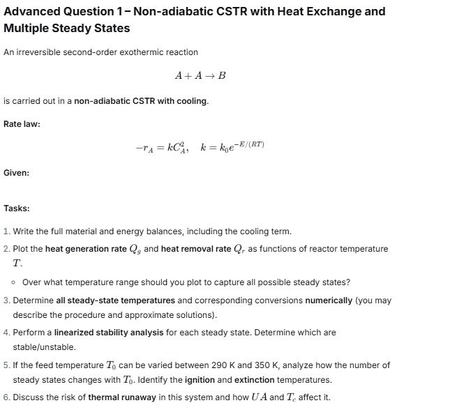
Give step-by-step solution with explanation and final answer:Advanced Question 1- Non-adiabatic CSTR with Heat Exchange and
Multiple Steady States
Anirreversible second-order exothermic reaction
A+A-B
is carried out in a non-adiabatic CSTR with cooling
Rate law:
ra =kC, k= koe FAD)
Givens
Tasks:
1. Write the full materi! and energy balances, including the cooling term.
2. Plot the heat generation rate (2, and heat removal rate Q, as functions of reactor temperature
T.
> Over what temperature range should you plot to capture all possible steady states?
3. Determine all steady-state temperatures and corresponding conversions numerically (you may
describe the procedure and approximate solutions).
4. Performa linearized stability analysis for each steady state. Determine which are
stable/unstable.
5.1f the feed temperature Tj can be varied between 290 K and 350 K, analyze how the number of
steady states changes with Tj. Identify the ignition and extinction temperatures.
6. Discuss the risk of thermal runaway in this system and how UA and T affect it.
Question:
Give step-by-step solution with explanation and final answer:Advanced Question 1- Non-adiabatic CSTR with Heat Exchange and
Multiple Steady States
Anirreversible second-order exothermic reaction
A+A-B
is carried out in a non-adiabatic CSTR with cooling
Rate law:
ra =kC, k= koe FAD)
Givens
Tasks:
1. Write the full materi! and energy balances, including the cooling term.
2. Plot the heat generation rate (2, and heat removal rate Q, as functions of reactor temperature
T.
> Over what temperature range should you plot to capture all possible steady states?
3. Determine all steady-state temperatures and corresponding conversions numerically (you may
describe the procedure and approximate solutions).
4. Performa linearized stability analysis for each steady state. Determine which are
stable/unstable.
5.1f the feed temperature Tj can be varied between 290 K and 350 K, analyze how the number of
steady states changes with Tj. Identify the ignition and extinction temperatures.
6. Discuss the risk of thermal runaway in this system and how UA and T affect it.
This is AI generated Response.
Asked by: Francis
Created at: 2026-01-17 09:01:13
Final Answer:
RenderedRaw Text
Did you like this answer?
Let's address each step-by-step for the **non-adiabatic CSTR with exothermic reaction and cooling**:
---
## 1. **Material and Energy Balances (with Cooling Term)**
### **Material Balance (Component A)**
For a CSTR:
\[
F(C_{A} - C_A) = V \cdot r_A
\]
where
- \( F \) = volumetric flow rate
- \( C_{A} \) = feed concentration of A
- \( C_A \) = exit concentration of A
- \( V \) = reactor volume
- \( r_A \) = rate of consumption of A
Given rate law:
\[
-r_A = k C_A^2 \\
k = k_ e^{-E/(RT)}
\]
So,
\[
F(C_{A} - C_A) = V k C_A^2
\]
---
### **Energy Balance (with heat exchange)**
\[
F \rho C_p (T_ - T) + (-\Delta H) V r_A = UA(T_c - T)
\]
where
- \( T_ \) = feed temperature
- \( T \) = reactor temperature
- \( \rho \), \( C_p \) = density, heat capacity of mixture
- \( \Delta H \) = heat of reaction (exothermic, so \( \Delta H < \))
- \( UA \) = overall heat transfer coefficient × area
- \( T_c \) = coolant temperature
Or, rearranged:
\[
F \rho C_p (T_ - T) + (-\Delta H) V k C_A^2 = UA(T_c - T)
\]
---
## 2. **Plotting \( Q_g \) and \( Q_r \) vs. \( T \)**
- **Heat Generation (\( Q_g \)):**
\[
Q_g = (-\Delta H) V k C_A^2
\]
In steady state, \( C_A \) depends on \( T \) via the material balance.
- **Heat Removal (\( Q_r \)):**
\[
Q_r = UA (T - T_c)
\]
(or, more generally, \( Q_r = F \rho C_p (T - T_) + UA (T - T_c) \), but often the first term is smaller and can be omitted for plotting).
#### **Temperature Range**
To capture **all steady states**, you should plot over a range that covers possible reactor operating temperatures, typically from slightly above \( T_c \) up to where \( k \) becomes very large (high conversion), e.g., 290 K to 450 K.
Look for intersections of \( Q_g \) and \( Q_r \): these are potential steady states.
---
## 3. **Numerical Steady-State Solutions**
You must **simultaneously solve** the material and energy balances for \( C_A \) and \( T \).
- Start with a guess for \( T \)
- Use the material balance to solve for \( C_A \):
\[
C_A = \frac{C_{A}}{1 + \frac{Vk}{F} C_A}
\]
(Which is quadratic; or iterate numerically)
- Plug back into energy balance, check if it balances.
- Adjust \( T \) and repeat to find all possible solutions.
**Each intersection in the \( Q_g \) and \( Q_r \) plot is a possible steady-state temperature.**
---
## 4. **Stability Analysis (Linearized)**
Linearize the energy balance around each steady state:
\[
\frac{dT}{dt} = \text{Net heat generation/removal}
\]
- Calculate \(\frac{d(Q_g - Q_r)}{dT}\) at each steady state.
- **Stable:** Slope is negative (\(\frac{d(Q_g - Q_r)}{dT} < \))
- **Unstable:** Slope is positive (\(\frac{d(Q_g - Q_r)}{dT} > \))
**Interpretation:**
If a small increase in \( T \) increases heat generation faster than removal, the system is unstable.
---
## 5. **Effect of Feed Temperature \( T_ \) (Ignition and Extinction)**
- Vary \( T_ \) and solve for steady states at each value.
- Low \( T_ \): Only low-\( T \) steady state (low conversion).
- As \( T_ \) increases, system may develop **multiple steady states** (S-shaped curve).
- **Ignition temperature:** Minimum \( T_ \) at which high-\( T \) steady state appears.
- **Extinction temperature:** Maximum \( T_ \) at which high-\( T \) state disappears.
---
## 6. **Thermal Runaway Risk and Effect of \( UA \), \( T_c \)**
- **Thermal Runaway:** If heat removal can't keep up with generation (e.g., \( UA \) too small, or \( T_c \) too high), system can jump to high-\( T \) runaway state.
- **Increasing \( UA \):** Increases heat removal, shifts \( Q_r \) up, reduces risk.
- **Lowering \( T_c \):** Increases driving force for heat removal, also reduces risk.
---
## **Summary Table**
| Step | Equation/Concept | Notes |
|------------|--------------------------------------------------------------------|-----------------------------------|
| Material | \( F(C_{A} - C_A) = V k C_A^2 \) | Second-order, exothermic |
| Energy | \( F \rho C_p (T_ - T) + (-\Delta H) V k C_A^2 = UA(T_c - T) \) | Cooling included |
| Plotting | \( Q_g = (-\Delta H) V k C_A^2 \), \( Q_r = UA(T - T_c) \) | Vs. \( T \), intersections = SS |
| Stability | \( \frac{d(Q_g - Q_r)}{dT} \) at SS | Negative: stable; Positive: unstable |
| \( T_ \) | Vary, note where multiple SS appear/disappear | Ignition/extinction points |
| Runaway | Small \( UA \), high \( T_c \): higher risk | |
---
### **Final Answer / Takeaways**
- **Multiple steady states** are possible due to exothermicity and cooling.
- **Stability** is determined by the sign of the slope at intersection points in the \( Q_g \) vs \( Q_r \) plot.
- **Thermal runaway** is a real risk; proper design (large \( UA \), low \( T_c \)) is essential.
- **Ignition/extinction** temperatures define the safe operating window.
---
### **Sketch Example Plot**
```plaintext
Q
^
| /
| /
| /
|----/
| /
| /
| /
+------------------> T
(Q_g curve) (Q_r line)
```
- **Three intersections** = three steady states (middle one unstable).
- **Change in UA or Tc** can reduce number of steady states (eliminate runaway).
---
If you need a detailed numerical example or code for plotting, let me know!
Question:
give me answer without using bullet points.
This is AI generated Response.
Asked by: Francis
Created at: 2026-01-17 09:14:18
Final Answer:
RenderedRaw Text
Did you like this answer?
# Step-by-Step Solution for Non-Adiabatic CSTR with Exothermic Reaction
## 1. Material and Energy Balances (with Cooling Term)
### Material Balance (Component A)
The material balance for a Continuous Stirred Tank Reactor (CSTR) is expressed as:
\[
F(C_{A} - C_A) = V \cdot r_A
\]
where \( F \) is the volumetric flow rate, \( C_A \) is the exit concentration of species A, \( C_{A} \) is the feed concentration, \( V \) is the reactor volume, and \( r_A \) is the rate of consumption of A.
From the rate law of the reaction \( A + A \rightarrow B \), we have:
\[
-r_A = k C_A^2
\]
with \( k = k_0 e^{-E/(RT)} \).
Substituting for \( r_A \), the material balance becomes:
\[
F(C_{A} - C_A) = V k C_A^2
\]
### Energy Balance (with Heat Exchange)
The energy balance for the CSTR can be written as:
\[
F \rho C_p (T_ - T) + (-\Delta H) V r_A = UA(T_c - T)
\]
where \( T_ \) is the feed temperature, \( T \) is the reactor temperature, \( \rho \) is the density, \( C_p \) is the heat capacity, \( \Delta H \) is the heat of reaction (negative for exothermic), \( UA \) is the overall heat transfer coefficient times the area, and \( T_c \) is the coolant temperature.
Rearranging, we get:
\[
F \rho C_p (T_ - T) + (-\Delta H) V k C_A^2 = UA(T_c - T)
\]
## 2. Plotting \( Q_g \) and \( Q_r \) vs. \( T \)
Heat generation (\( Q_g \)) is given by:
\[
Q_g = (-\Delta H) V k C_A^2
\]
and heat removal (\( Q_r \)):
\[
Q_r = UA(T - T_c)
\]
To capture all possible steady states, plot over a temperature range from slightly above \( T_c \) to around 450 K. This range allows visualization of intersections between \( Q_g \) and \( Q_r \), indicating potential steady-state temperatures.
## 3. Numerical Steady-State Solutions
To find steady-state solutions, simultaneously solve the material and energy balances for \( C_A \) and \( T \). Start with an initial guess for \( T \), use the material balance to solve for \( C_A \):
\[
C_A = \frac{C_{A}}{1 + \frac{Vk}{F} C_A}
\]
This quadratic equation can be solved iteratively or numerically. Substitute \( C_A \) back into the energy balance and check for consistency. Repeat this process to find all steady-state temperatures corresponding to each intersection point in the \( Q_g \) and \( Q_r \) plot.
## 4. Stability Analysis (Linearized)
Perform a linear stability analysis by linearizing the energy balance around each steady state:
\[
\frac{dT}{dt} = \text{Net heat generation/removal}
\]
Calculate the derivative \(\frac{d(Q_g - Q_r)}{dT}\) at each steady state. A negative slope indicates stability, while a positive slope indicates instability.
## 5. Effect of Feed Temperature \( T_ \)
Vary \( T_ \) and analyze the resulting steady states. At lower \( T_ \), only a low-temperature steady state exists. As \( T_ \) increases, multiple steady states may form. The ignition temperature is the minimum \( T_ \) where a high-temperature steady state appears, while the extinction temperature is the maximum \( T_ \) beyond which the high-temperature state disappears.
## 6. Thermal Runaway Risk and Effects of \( UA \) and \( T_c \)
Thermal runaway can occur if the heat generation exceeds heat removal capacity, such as when \( UA \) is too low or \( T_c \) is too high. Increasing \( UA \) enhances heat removal, reducing the risk of runaway. Lowering \( T_c \) increases the driving force for heat removal, also mitigating risk.
---
## Summary
A non-adiabatic CSTR with an exothermic reaction exhibits multiple steady states, influenced by the heat generation and removal dynamics. Stability analysis reveals the conditions under which these states are stable or unstable. Variations in feed temperature \( T_ \) impact the number of steady states, defining critical ignition and extinction points. Careful design considerations regarding heat transfer coefficients and coolant temperatures are necessary to prevent thermal runaway.
VIPSolutions focuses on clear, step‑by‑step explanations so you can learn quickly. Whether you need an AI‑generated walkthrough or a short hint to get unstuck, each solution is organized for fast reading and easy review later.
Search similar questions, compare approaches, and bookmark the best answers for revision. Our goal is simple: quick, reliable study help that feels natural—not noisy.
 VIPSolutions
 Advanced Question 1- Non-adiabatic CSTR with Heat Exchange and
Multiple Steady States
Anirreversible second-order exothermic reaction
A+A-B
is carried out in a non-adiabatic CSTR with cooling
Rate law:
ra =kC, k= koe FAD)
Givens
Tasks:
1. Write the full materi! and energy balances, including the cooling term.
2. Plot the heat generation rate (2, and heat removal rate Q, as functions of reactor temperature
T.
> Over what temperature range should you plot to capture all possible steady states?
3. Determine all steady-state temperatures and corresponding conversions numerically (you may
describe the procedure and approximate solutions).
4. Performa linearized stability analysis for each steady state. Determine which are
stable/unstable.
5.1f the feed temperature Tj can be varied between 290 K and 350 K, analyze how the number of
steady states changes with Tj. Identify the ignition and extinction temperatures.
6. Discuss the risk of thermal runaway in this system and how UA and T affect it.