 VIPSolutions
Act like a helpful tutor and exlain step-by-step solution with explanation and final answer:Problem 1. Given initial anisotropic boundary constraints governing spatial deformation within a heterogeneous granular continuum, a rigorous mathematical formulation of the macroscopic yield criterion is strictly necessary. Assuming rigid base immobility under transient deviatoric loading conditions, structural yield limits require immediate analytical deduction. Under continuous kinematic loading conditions across arbitrary control volumes, generalized non-associative plasticity flow rules demand precise algebraic establishment. Principal invariant directions mapping initial to spatial configurations mandate a complete tensor derivation before progressing further. Paynamic H,(j0) 7 Sr yd a « Utilizing the designated yield surface parameters, an explicit derivation of the three-dimensional non-associative flow rule partial differential equations becomes indispensable for describing the rate of plastic strain evolution. « Uliitzing the designated yield surface montors, an explicit derivation of stress of plastic strain evolution. « Integrate the comparision exscontanic nesis docaine flow direction for rate of plastic strain direction. » Considering the derived flow rule, the establishment of the corresponding fourth-order spatial tangent stiffness tensor necessitates careful analytical construction to capture the instantaneous stress-strain response. « Considere the reessmatic for for plastic stress-strain response. « Consider the instantaneous plastic flow acadomaf tra analytics directions. Problem 2. Because of asymmetric mass distribution coupled with non-linear dissipative mechanisms within the granular matrix, a governing differential equation of motion for the coupled plastic wave propagation requires precise derivation. Representing multi-variable limit cycle predictions within continuous state-space matrix transformations, a rigorous describing function must be established. « A complete mathematical formulation of the governing partial differential equations for 3D elastoplastic wave propagation, integrating the non-associative flow rule and tangent stiffness tensor previously derived, is required. Integrates the semulative flow after elastoplastic wave propagation. ® Decvmure the non-associatic rule and tangent stiffness tensor. « An analytical derivation of the dispersion relations for coupled shear and compressional waves under the plastic regime must be formulated. « Formulate on ensotion of the dispersion mistis regiines. « Formulate an eesotion of the plastiz and compressional waves. « The establishment of the energy dissipation rate tensor utilizing the derived plastic strain rate vectors and the yield function is necessary for energy conservation analysis. « Formulaten of the energy dissipation fire energy caie analysis. « Formulate rate eatood yield function is necessary or the energy dissipation. Problem 3. Upon integrating turbulent kinetic energy dissipation vectors along spatial boundary layers within the saturated granular media, fundamental Reynolds stress transport tensors dictate analytical reconstruction. « A rigorous derivation of the 3D Biot poroelastodynamics equations, incorporating the plastic dissipation terms and the effective stress principle, must be established. « The formulation of the corresponding boundary integral equations for dynamic soil-structure interaction utilizing the derived elastodynamic Green's functions is required. « An analytical evaluation of the spatial attenuation coefficients for the coupled wave modes within the poroelasto- plastic medium demands precise mathematical construction. © The derivation of the steady-state response functions for the granular continuum under harmonic excitation requires careful algebraic development.
Question:
Act like a helpful tutor and exlain step-by-step solution with explanation and final answer: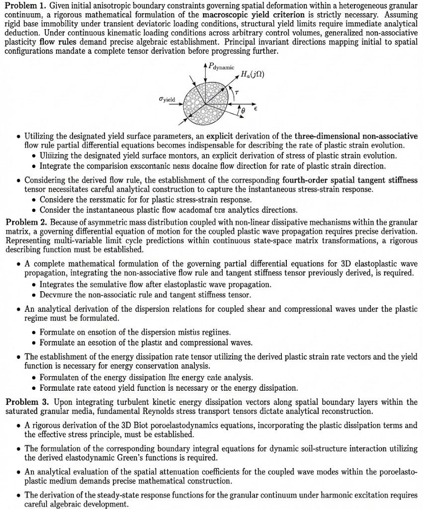 Problem 1. Given initial anisotropic boundary constraints governing spatial deformation within a heterogeneous granular
continuum, a rigorous mathematical formulation of the macroscopic yield criterion is strictly necessary. Assuming
rigid base immobility under transient deviatoric loading conditions, structural yield limits require immediate analytical
deduction. Under continuous kinematic loading conditions across arbitrary control volumes, generalized non-associative
plasticity flow rules demand precise algebraic establishment. Principal invariant directions mapping initial to spatial
configurations mandate a complete tensor derivation before progressing further.
Paynamic
H,(j0)
7 Sr
yd
a
« Utilizing the designated yield surface parameters, an explicit derivation of the three-dimensional non-associative
flow rule partial differential equations becomes indispensable for describing the rate of plastic strain evolution.
« Uliitzing the designated yield surface montors, an explicit derivation of stress of plastic strain evolution.
« Integrate the comparision exscontanic nesis docaine flow direction for rate of plastic strain direction.
» Considering the derived flow rule, the establishment of the corresponding fourth-order spatial tangent stiffness
tensor necessitates careful analytical construction to capture the instantaneous stress-strain response.
« Considere the reessmatic for for plastic stress-strain response.
« Consider the instantaneous plastic flow acadomaf tra analytics directions.
Problem 2. Because of asymmetric mass distribution coupled with non-linear dissipative mechanisms within the granular
matrix, a governing differential equation of motion for the coupled plastic wave propagation requires precise derivation.
Representing multi-variable limit cycle predictions within continuous state-space matrix transformations, a rigorous
describing function must be established.
« A complete mathematical formulation of the governing partial differential equations for 3D elastoplastic wave
propagation, integrating the non-associative flow rule and tangent stiffness tensor previously derived, is required.
Integrates the semulative flow after elastoplastic wave propagation.
® Decvmure the non-associatic rule and tangent stiffness tensor.
« An analytical derivation of the dispersion relations for coupled shear and compressional waves under the plastic
regime must be formulated.
« Formulate on ensotion of the dispersion mistis regiines.
« Formulate an eesotion of the plastiz and compressional waves.
« The establishment of the energy dissipation rate tensor utilizing the derived plastic strain rate vectors and the yield
function is necessary for energy conservation analysis.
« Formulaten of the energy dissipation fire energy caie analysis.
« Formulate rate eatood yield function is necessary or the energy dissipation.
Problem 3. Upon integrating turbulent kinetic energy dissipation vectors along spatial boundary layers within the
saturated granular media, fundamental Reynolds stress transport tensors dictate analytical reconstruction.
« A rigorous derivation of the 3D Biot poroelastodynamics equations, incorporating the plastic dissipation terms and
the effective stress principle, must be established.
« The formulation of the corresponding boundary integral equations for dynamic soil-structure interaction utilizing
the derived elastodynamic Green's functions is required.
« An analytical evaluation of the spatial attenuation coefficients for the coupled wave modes within the poroelasto-
plastic medium demands precise mathematical construction.
© The derivation of the steady-state response functions for the granular continuum under harmonic excitation requires
careful algebraic development.
Asked by: Francis
Created at: 2026-02-26 21:26:54
Final Answer:
Question:
give me answer in simple way
Asked by: Francis
Created at: 2026-02-26 21:29:14
Final Answer:
📢 Instructions:
- Ask anything relatd to above question only.
- For new Question goto :