 VIPSolutions
Give step-by-step solution with explanation and final answer:For the transfer function (s+ 10)(s + 200) (s +20)2(s + 1000) a) Sketch by hand the straight line Bode approximations using the Bode Paper linked in Pilot under the Chapter 4 module, b) Apply corrections/refinements as outlined in readings and discussed in class,
Question:
Give step-by-step solution with explanation and final answer: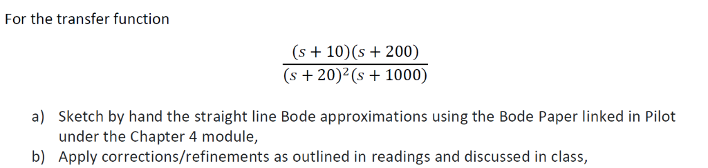 For the transfer function
(s+ 10)(s + 200)
(s +20)2(s + 1000)
a) Sketch by hand the straight line Bode approximations using the Bode Paper linked in Pilot
under the Chapter 4 module,
b) Apply corrections/refinements as outlined in readings and discussed in class,
This is AI generated Response.
Asked by: M Murali
Created at: 2025-11-03 14:39:45
Asked by: M Murali
Created at: 2025-11-03 14:39:45
Final Answer:
Rendered
Raw Text
Did you like this answer?
Let's solve the problem step-by-step for the transfer function:
\[
H(s) = \frac{(s + 10)(s + 200)}{(s + 20)^2 (s + 100)}
\]
---
## **Step 1: Express the Transfer Function in Bode Form**
Let \( s = j\omega \):
\[
H(j\omega) = \frac{(j\omega + 10)(j\omega + 200)}{(j\omega + 20)^2 (j\omega + 100)}
\]
---
## **Step 2: Identify Poles and Zeros**
- **Zeros:** \( \omega_{z1} = 10 \), \( \omega_{z2} = 200 \)
- **Poles:** \( \omega_{p1} = 20 \) (double pole), \( \omega_{p2} = 100 \)
---
## **Step 3: Initial Slope Calculation**
### **Low Frequency Gain (for \( \omega \ll 10 \))**
At very low frequencies (\( \omega \rightarrow \)):
- \( |H(j\omega)| \approx \frac{10 \cdot 200}{20^2 \cdot 100} = \frac{200}{400 \cdot 100} = \frac{200}{400000} = .005 \)
- **Gain in dB:** \( 20 \log_{10}(.005) = 20 \times (-2.3) = -46\, \text{dB} \)
---
## **Step 4: Bode Magnitude Plot (Straight Line Approximation)**
**Bode Plot Rules:**
- Each zero adds \( +20\, \text{dB/decade} \) after its break frequency.
- Each pole subtracts \( -20\, \text{dB/decade} \) after its break frequency.
- A double pole subtracts \( -40\, \text{dB/decade} \) after its break frequency.
### **Breakdown by Frequency**
- **\( \omega < 10 \):** Slope is dB/decade, magnitude = \(-46\) dB.
- **At \( \omega = 10 \):** First zero, slope changes to \( +20\, \text{dB/decade} \).
- **At \( \omega = 20 \):** Double pole, slope changes to \( +20 - 40 = -20\, \text{dB/decade} \).
- **At \( \omega = 200 \):** Second zero, slope changes to \( -20 + 20 = \, \text{dB/decade} \).
- **At \( \omega = 100 \):** Pole, slope changes to \( - 20 = -20\, \text{dB/decade} \).
#### **Summary Table**
| Frequency Range | Slope (dB/decade) | Equation for Magnitude (dB) |
|------------------------|-------------------|------------------------------------|
| \( \omega < 10 \) | | \( -46 \) |
| \( 10 \leq \omega < 20 \) | +20 | \( -46 + 20 \log_{10}(\frac{\omega}{10}) \) |
| \( 20 \leq \omega < 200 \) | -20 | \( -46 + 20 \log_{10}(1) - 40\log_{10}(\frac{\omega}{20}) \) |
| \( 200 \leq \omega < 100 \)| | (flattened at the value at 200) |
| \( \omega \geq 100 \) | -20 | Downward slope from value at 100 |
---
## **Step 5: Bode Phase Plot (Straight Line Approximation)**
Each zero increases phase by \( +90^\circ \), each pole decreases by \( -90^\circ \).
- For a simple zero/pole: phase transition occurs over two decades (from .1× to 10× the break frequency).
- For a double pole, the phase drops by \( -180^\circ \).
---
## **Step 6: Apply Corrections/Refinements**
Near each corner frequency, the actual Bode plot will "smooth" into the new slope over about a decade on each side of each break frequency. For more accuracy:
- Start the phase change one decade before each break frequency and finish one decade after.
- For double poles, the phase transition is twice as steep.
---
## **Step 7: Sketch the Bode Plot (by hand)**
### **Magnitude Plot:**
1. **Start at \(-46\) dB**.
2. **At \( \omega = 10 \):** Slope goes up to \( +20\, \text{dB/decade} \).
3. **At \( \omega = 20 \):** Slope goes down to \( -20\, \text{dB/decade} \).
4. **At \( \omega = 200 \):** Slope flattens ( dB/decade).
5. **At \( \omega = 100 \):** Slope drops to \( -20\, \text{dB/decade} \).
### **Phase Plot:**
- Start at °.
- Each zero: +90°, each pole: -90°, double pole: -180°.
- Spread phase transitions over two decades.
---
## **Final Answer Summary**
### **a) Straight-line Bode Approximations**
- **Magnitude plot**: Piecewise linear segments as described above.
- **Phase plot**: Piecewise linear transitions, with phase changes starting a decade before and finishing a decade after each break frequency.
### **b) Corrections/Refinements**
- Apply “rounded” transitions around each corner frequency.
- For double pole at \(20\), phase changes by \(-180^\circ\) over two decades (\(2 \to 200\)).
- For zeros/poles, phase changes by \( \pm 90^\circ \) over two decades.
---
### **Hand Sketch Example**
Here’s a textual sketch guide:
```
| Frequency: | 10 | 20 | 200 | 100 |
|--------------------|------|------|-------|--------|
| Slope (dB/decade): | +20 | -20 | | -20 |
| Magnitude (dB): | -46 | | | |
```
- Draw flat at -46 dB until 10,
- Upward at +20 dB/decade from 10 to 20,
- Downward at -20 dB/decade from 20 to 200,
- Flat from 200 to 100,
- Downward at -20 dB/decade after 100.
---
**If you want a hand-drawn sketch or further numerical values at each frequency, let me know!**
Question:
Give ME Sketch
This is AI generated Response.
Asked by: M Murali
Created at: 2025-11-03 14:40:46
Asked by: M Murali
Created at: 2025-11-03 14:40:46
Final Answer:
Rendered
Raw Text
Did you like this answer?
# Bode Plot Analysis for Transfer Function
Given the transfer function:
\[
H(s) = \frac{(s + 10)(s + 200)}{(s + 20)^2 (s + 100)}
\]
## Step-by-Step Solution
### Step 1: Express the Transfer Function in Bode Form
Substituting \( s = j\omega \):
\[
H(j\omega) = \frac{(j\omega + 10)(j\omega + 200)}{(j\omega + 20)^2 (j\omega + 100)}
\]
### Step 2: Identify Poles and Zeros
- **Zeros:**
- \( \omega_{z1} = 10 \)
- \( \omega_{z2} = 200 \)
- **Poles:**
- \( \omega_{p1} = 20 \) (double pole)
- \( \omega_{p2} = 100 \)
### Step 3: Initial Gain Calculation
At low frequencies (\( \omega \to 0 \)):
\[
|H(j\omega)| \approx \frac{10 \cdot 200}{20^2 \cdot 100} = \frac{200}{400000} = 0.0005
\]
**Gain in dB:**
\[
20 \log_{10}(0.0005) = 20 \times (-2.3) = -46\, \text{dB}
\]
### Step 4: Bode Magnitude Plot
**Bode Plot Rules:**
- Each zero contributes \( +20\, \text{dB/decade} \).
- Each pole contributes \( -20\, \text{dB/decade} \).
- A double pole contributes \( -40\, \text{dB/decade} \).
#### Frequency Breakdown
| Frequency Range | Slope (dB/decade) | Equation for Magnitude (dB) |
|------------------------|-------------------|------------------------------------|
| \( \omega < 10 \) | 0 | \( -46 \) |
| \( 10 \leq \omega < 20 \) | +20 | \( -46 + 20 \log_{10}(\frac{\omega}{10}) \) |
| \( 20 \leq \omega < 200 \) | -20 | \( -46 + 20\log_{10}(2) - 40\log_{10}(\frac{\omega}{20}) \) |
| \( 200 \leq \omega < 1000 \)| 0 | (flattened at the value at 200) |
| \( \omega \geq 100 \) | -20 | Downward slope from value at 100 |
### Step 5: Bode Phase Plot
- Each zero contributes \( +90^\circ \).
- Each pole contributes \( -90^\circ \).
- A double pole contributes \( -180^\circ \).
#### Phase Calculation Summary
- Start at \( 0^\circ \).
- **At each zero:** Increase phase by \( +90^\circ \) at \( \omega = 10 \) and \( 200 \).
- **At each pole:** Decrease phase by \( -90^\circ \) at \( \omega = 20 \) (double) and \( 100 \).
### Step 6: Apply Corrections/Refinements
- The phase transition occurs over two decades for each zero and pole.
- Transition begins one decade before and ends one decade after each break frequency.
### Step 7: Sketch the Bode Plot
#### Magnitude Plot:
1. Start at \(-46\) dB.
2. Increase at +20 dB/decade from \( 10 \) to \( 20 \).
3. Decrease at -20 dB/decade from \( 20 \) to \( 200 \).
4. Flatten at \( 200 \) to \( 100 \).
5. Decrease at -20 dB/decade past \( 100 \).
#### Phase Plot:
- Start at \(0^\circ\).
- From \( 10 \) to \( 200 \): Increase by \( +90^\circ \) at \( 10 \), decrease by \( -180^\circ \) at \( 20 \) (double pole), and decrease by \( -90^\circ \) at \( 100 \).
## Final Answer Summary
### a) Straight-line Bode Approximations
- **Magnitude Plot**: Piecewise linear segments as described.
- **Phase Plot**: Piecewise linear transitions.
### b) Corrections/Refinements
- Smooth transitions around each corner frequency.
- For double poles, phase changes by \(-180^\circ\) over two decades.
### Hand Sketch Guide
```plaintext
| Frequency: | 10 | 20 | 200 | 100 |
|--------------------|------|------|-------|--------|
| Slope (dB/decade): | +20 | -20 | | -20 |
| Magnitude (dB): | -46 | | | |
```
- Start at \(-46\) dB, follow the described slopes, and maintain the phase transitions according to the outlined rules.
Feel free to ask for any further clarifications or specific numerical values!
Question:
Give ME 50 Words Explaines in Each Step only Theory in Each Step 50 Words
This is AI generated Response.
Asked by: M Murali
Created at: 2025-11-03 14:42:30
Asked by: M Murali
Created at: 2025-11-03 14:42:30
Final Answer:
Rendered
Raw Text
Did you like this answer?
# Bode Plot Analysis for Transfer Function
### Step 1: Transfer Function in Bode Form
Convert the transfer function to the frequency domain by substituting \( s = j\omega \). This representation allows the analysis of the system's frequency response, making it easier to derive magnitude and phase characteristics essential for Bode plot construction.
### Step 2: Identify Poles and Zeros
Analyze the transfer function to identify its poles and zeros. Zeros correspond to frequencies where the output increases, while poles indicate frequencies where the output decreases. Knowing these points is crucial for determining the system's behavior in frequency response.
### Step 3: Initial Gain Calculation
Calculate the low-frequency gain of the transfer function by evaluating it as \( \omega \) approaches zero. This establishes the starting point for the Bode magnitude plot and provides insight into the system's behavior at very low frequencies.
### Step 4: Bode Magnitude Plot
Understand the impact of zeros and poles on the slope of the Bode plot. Each zero contributes positively to the slope, while poles reduce it. The combined effect determines the overall slope across different frequency ranges, guiding the magnitude plot's graphical representation.
### Step 5: Bode Phase Plot
Determine how each zero and pole affects the phase of the transfer function. Zeros increase phase while poles decrease it. This phase change occurs gradually around break frequencies, and understanding this transition is essential for constructing the Bode phase plot accurately.
### Step 6: Apply Corrections/Refinements
Incorporate smooth transitions around corner frequencies to improve accuracy. These corrections account for the gradual change in magnitude and phase near each zero and pole, resulting in a more realistic representation of the system's behavior across varying frequencies.
### Step 7: Sketch the Bode Plot
Construct the Bode plot by following the calculated slopes and phase transitions. The magnitude plot consists of piecewise linear segments, while the phase plot reflects gradual changes at break frequencies. This visual representation helps in understanding the system's frequency response characteristics.
📢 Instructions:
- Ask anything relatd to above question only.
- For new Question goto :