 VIPSolutions
give answer in 2 step with explanation at the end of each step and final answer at the end:9. For a system of discrete point particles the energy-momentum tensor takes the form 2p” ©) (@ ab pall ihin — wll Tyv=) ot 89 (x — x@), (1.173) a where the index a labels the different particles. Show that, for a dense collection of particles with isotropically distributed velocities, we can smooth over the individual particle worldlines to obtain the perfect-fluid energy-momentum tensor (1.114). A a CE ET sg I Ee YE
Question:
give answer in 2 step with explanation at the end of each step and final answer at the end: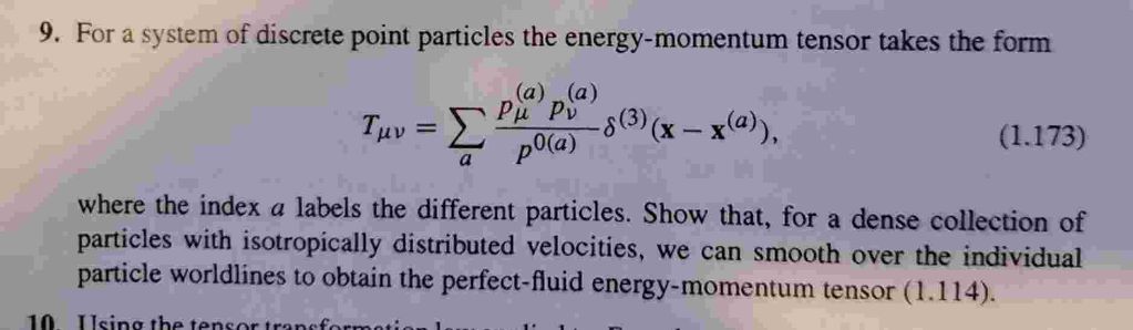 9. For a system of discrete point particles the energy-momentum tensor takes the form
2p” ©) (@
ab pall ihin — wll
Tyv=) ot 89 (x — x@), (1.173)
a
where the index a labels the different particles. Show that, for a dense collection of
particles with isotropically distributed velocities, we can smooth over the individual
particle worldlines to obtain the perfect-fluid energy-momentum tensor (1.114).
A a CE ET sg I Ee YE
This is AI generated Response.
Asked by: Rahulkumar
Created at: 2025-10-07 03:55:47
Asked by: Rahulkumar
Created at: 2025-10-07 03:55:47
Final Answer:
Rendered
Raw Text
Did you like this answer?
### Step 1: Write the Discrete Energy-Momentum Tensor and Interpret the Terms
Given for a system of discrete point particles:
\[
T^{\mu\nu} = \sum_a \frac{p^\mu_{(a)} p^\nu_{(a)}}{p^_{(a)}} \delta^{(3)}(\vec{x} - \vec{x}^{(a)})
\]
- Here, \(a\) labels particles, \(p^\mu_{(a)}\) is the 4-momentum of particle \(a\), and \(\delta^{(3)}(\vec{x} - \vec{x}^{(a)})\) localizes the tensor at the position of each particle.
**Explanation:**
This tensor describes energy and momentum density at each point in space due to all particles. It is highly "spiky" (not smooth), since each particle only contributes at its exact location.
---
### Step 2: Smooth to a Continuous Fluid Description
For a **dense collection** of particles with **isotropically distributed velocities**, replace sums by integrals over a continuous distribution function \(f(\vec{x}, \vec{p})\):
\[
T^{\mu\nu}(\vec{x}) = \int \frac{d^3 p}{p^} f(\vec{x}, \vec{p}) p^\mu p^\nu
\]
- For an **isotropic distribution**, the momentum average satisfies:
- \(\langle p^i p^j \rangle \propto \delta^{ij}\), so off-diagonal spatial terms vanish.
- For a **perfect fluid**, the energy-momentum tensor is:
\[
T^{\mu\nu} = (\rho + P) u^\mu u^\nu + P \eta^{\mu\nu}
\]
where \(\rho\) is energy density, \(P\) is pressure, and \(u^\mu\) is the fluid 4-velocity.
**Explanation:**
The integral form is smooth and, due to isotropy, matches the perfect-fluid form: energy and momentum are distributed smoothly, and off-diagonal terms vanish, leaving only energy density and isotropic pressure.
---
### **Final Answer**
**For a dense collection of particles with isotropically distributed velocities, the sum over individual particle worldlines can be replaced by an integral over a smooth distribution function, which yields the perfect-fluid energy-momentum tensor.**
Question:
Please solve step by step
This is AI generated Response.
Asked by: Rahulkumar
Created at: 2025-10-07 03:56:48
Asked by: Rahulkumar
Created at: 2025-10-07 03:56:48
Final Answer:
Rendered
Raw Text
Did you like this answer?
### Step 1: Write the Discrete Energy-Momentum Tensor and Interpret the Terms
Given the discrete energy-momentum tensor for point particles:
\[
T^{\mu\nu} = \sum_a \frac{p^\mu_{(a)} p^\nu_{(a)}}{p^{}_{(a)}} \delta^{(3)}(\vec{x} - \vec{x}^{(a)})
\]
- **Terms Explained**:
- \(a\): Index labeling individual particles.
- \(p^\mu_{(a)}\): 4-momentum of particle \(a\), comprising energy and momentum.
- \(\delta^{(3)}(\vec{x} - \vec{x}^{(a)})\): 3-dimensional delta function, which localizes the contribution of each particle to its specific position.
**Explanation:**
This tensor reflects how energy and momentum are distributed in space due to a collection of particles. The use of the delta function indicates that contributions are concentrated at the exact locations of the particles, resulting in a "spiky" distribution rather than a smooth one.
---
### Step 2: Smooth to a Continuous Fluid Description
For a **dense collection** of particles with **isotropically distributed velocities**, we transition from the sum to an integral over a continuous distribution function \(f(\vec{x}, \vec{p})\):
\[
T^{\mu\nu}(\vec{x}) = \int \frac{d^3 p}{p} f(\vec{x}, \vec{p}) p^\mu p^\nu
\]
- **Isotropic Distribution**:
- Average momentum components satisfy: \(\langle p^i p^j \rangle \propto \delta^{ij}\), meaning momentum is evenly distributed in all directions.
- **Perfect Fluid Form**:
- The energy-momentum tensor for a perfect fluid is defined as:
\[
T^{\mu\nu} = (\rho + P) u^\mu u^\nu + P \eta^{\mu\nu}
\]
where:
- \(\rho\): Energy density.
- \(P\): Pressure.
- \(u^\mu\): 4-velocity of the fluid.
**Explanation:**
This integral reduces the discrete particles to a smooth energy and momentum distribution across space. The isotropic nature ensures that the contributions to the tensor match the structure of a perfect fluid, with only diagonal terms remaining.
---
### **Final Answer**
**Thus, for a dense collection of particles with isotropically distributed velocities, the sum over individual particle worldlines can be replaced by an integral over a smooth distribution function, yielding the perfect-fluid energy-momentum tensor.**
📢 Instructions:
- Ask anything relatd to above question only.
- For new Question goto :