 VIPSolutions
give answer in 2 step with explanation at the end of each step and final answer at the end:What is your interpretation of the initial-boundary-value problem? PDE u, = au, 0
Question:
give answer in 2 step with explanation at the end of each step and final answer at the end: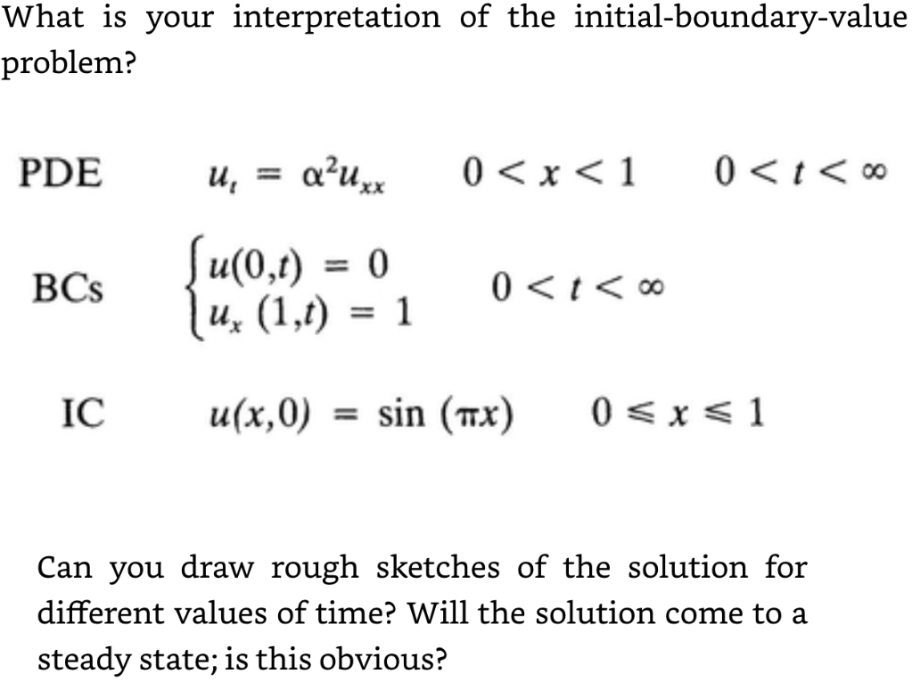 What is your interpretation of the initial-boundary-value
problem?
PDE u, = au, 0
This is AI generated Response.
Asked by: Pagal
Created at: 2025-09-02 02:37:47
Asked by: Pagal
Created at: 2025-09-02 02:37:47
Final Answer:
Rendered
Raw Text
Did you like this answer?
### Step 1: Interpretation of the Problem
**Explanation:**
- The given PDE is the heat (diffusion) equation: \( u_t = \alpha^2 u_{xx} \), describing how temperature (or another diffusing quantity) evolves over time on the interval \( 0 < x < 1 \).
- Boundary conditions (BCs):
- \( u(0, t) = 0 \): The value at the left end is always zero.
- \( u_x(1, t) = 1 \): The spatial derivative (slope) at the right end is always 1, which is a Neumann boundary condition.
- Initial condition (IC):
- \( u(x, 0) = \sin(\pi x) \): The initial temperature profile is a sine wave.
**Interpretation:**
This problem models heat diffusion in a rod of length 1, where the left end is kept at zero temperature, and the right end has a fixed heat flux (slope). The rod starts with a sine-shaped temperature distribution.
---
### Step 2: Solution Behavior and Steady State
**Explanation:**
- **Early times (\( t \approx 0 \))**: The solution matches the initial sine wave, \( u(x, 0) = \sin(\pi x) \).
- **As time increases**: The solution smooths out due to diffusion, and the boundary conditions start to dominate the shape.
- **Long time (\( t \to \infty \)):** The system reaches a steady-state solution \( u_s(x) \) where \( u_t = 0 \), so \( u_{xx} = 0 \). Integrating twice and applying the BCs:
- \( u_s(0) = 0 \)
- \( u_s'(1) = 1 \)
- Thus, the steady-state solution is a straight line: \( u_s(x) = x \).
**Sketches:**
- At \( t = 0 \): Sine curve from 0 to 0.
- For small \( t \): The curve starts to flatten, especially near \( x = 1 \), to meet the boundary slope.
- For large \( t \): The curve approaches a straight line from (0,0) to (1,1).
**Steady State:**
Yes, the solution will come to a steady state, and it is obvious because the heat equation dissipates initial shapes, and the boundary conditions dictate a unique steady state.
---
### **Final Answer:**
**The initial-boundary-value problem describes heat diffusion in a rod with one fixed end and one end with a fixed heat flux. The solution starts as a sine wave and evolves over time to a straight line (\( u_s(x) = x \)), which is the steady state.**
Question:
All parts solved give answer in 2 step with explanation at the end of each step and final answer at the end:
This is AI generated Response.
Asked by: Pagal
Created at: 2025-09-02 02:38:35
Asked by: Pagal
Created at: 2025-09-02 02:38:35
Final Answer:
Rendered
Raw Text
Did you like this answer?
### Step 1: Interpretation of the Problem
**Explanation:**
The PDE \( u_t = \alpha^2 u_{xx} \) models heat diffusion along a one-dimensional rod of length 1.
- Boundary conditions:
- \( u(0, t) = 0 \) indicates the left end of the rod is held at zero temperature.
- \( u_x(1, t) = 1 \) specifies a constant heat flux (gradient) at the right end.
- Initial condition: \( u(x, 0) = \sin(\pi x) \) means the initial temperature distribution is a sine wave along the rod.
**Interpretation:**
This setup describes how an initial sine-shaped temperature distribution evolves over time, with fixed temperature at one end and a constant heat flux at the other, illustrating a diffusion process influenced by these boundary conditions.
---
### Step 2: Solution Behavior and Steady State
**Explanation:**
- At early times, the solution resembles the initial sine wave.
- As time progresses, diffusion causes the temperature profile to smooth out, influenced by boundary conditions.
- The steady state occurs when \( u_t = 0 \), leading to \( u_{xx} = 0 \). Integrating twice:
\[
u_s(x) = A x + B
\]
Applying BCs:
- \( u_s(0) = 0 \Rightarrow B=0 \).
- \( u_x(1) = A = 1 \).
So, the steady state is \( u_s(x) = x \).
**Sketches:**
- Initially: sine wave \( \sin(\pi x) \).
- With time: the profile becomes flatter near \( x=0 \) and adjusts near \( x=1 \) due to the boundary flux.
- Long-term: the temperature profile approaches the straight line \( u(x) = x \).
**Conclusion:**
Yes, the solution will tend to the steady state \( u(x) = x \), as it is consistent with the boundary conditions and the nature of diffusion.
---
### **Final Answer:**
The problem models heat diffusion in a rod with fixed temperature at one end and constant heat flux at the other. The solution starts as a sine wave and evolves over time toward a steady state linear profile \( u(x) = x \).
Question:
BCS [u(0,t) = 0 (ux (1,t) = 1 0
This is AI generated Response.
Asked by: Pagal
Created at: 2025-09-02 02:41:13
Asked by: Pagal
Created at: 2025-09-02 02:41:13
Final Answer:
Rendered
Raw Text
Did you like this answer?
**Step 1: Understanding the Boundary Conditions and Steady State**
**Explanation:**
The boundary conditions are:
- \( u(0,t) = 0 \): The temperature at \( x=0 \) is held fixed at zero for all times.
- \( u_x(1,t) = 1 \): The heat flux (or spatial derivative) at \( x=1 \) is held constant at 1 for all times.
In the long-term (steady state), the time derivative \( u_t \) becomes zero, so the PDE reduces to:
\[
u_{xx} = 0
\]
whose general solution is:
\[
u_s(x) = A x + B
\]
Applying the boundary conditions for the steady state:
- At \( x=0 \):
\[
u_s(0) = B = 0
\]
- At \( x=1 \):
\[
u_x(1) = A = 1
\]
Thus, the steady-state solution is:
\[
\boxed{
u_s(x) = x
}
\]
---
**Step 2: Interpretation of the Solution Behavior**
**Explanation:**
- The boundary condition \( u(0,t) = 0 \) fixes the temperature at the left end at zero.
- The boundary condition \( u_x(1,t) = 1 \) imposes a constant heat flux at the right end, meaning heat flows into the domain at a steady rate.
- Over time, the solution will evolve from any initial condition toward the steady state \( u_s(x) = x \), which satisfies both boundary conditions.
**Will the solution come to a steady state?**
Yes. The heat equation with these boundary conditions is well-posed and dissipative, so the solution will tend to the steady state \( u(x) = x \).
**Sketching the solution:**
- Initially, the solution might vary depending on the initial condition, but as \( t \to \infty \), it approaches the straight line \( u(x) = x \).
- The profile will gradually smooth out and adjust to meet the boundary conditions, approaching the steady state from below or above depending on initial data.
---
### **Final Answer:**
The boundary conditions specify a fixed temperature at \( x=0 \) and a constant heat flux at \( x=1 \). The solution of the PDE will evolve over time from initial conditions toward the steady state \( u(x) = x \), satisfying both boundary conditions, with the temperature profile becoming a straight line from 0 at the left end to a slope of 1 at the right end.
📢 Instructions:
- Ask anything relatd to above question only.
- For new Question goto :